https://doi.org/10.5194/essd-9-471-2017 © Author(s) 2017. This work is distributed under the Creative Commons Attribution 3.0 License.
Using ERA-Interim reanalysis for creating datasets
of energy-relevant climate variables
Philip D. Jones1,4, Colin Harpham1, Alberto Troccoli2,5, Benoit Gschwind3, Thierry Ranchin3,
Lucien Wald3, Clare M. Goodess1, and Stephen Dorling2
1Climatic Research Unit (CRU), School of Environmental Sciences,University of East Anglia,
Norwich, NR4 7TJ, UK
2School of Environmental Sciences, University of East Anglia, Norwich, NR4 7TJ, UK
3MINES ParisTech, PSL Research University, O.I.E. – Centre Observation, Impacts, Energy,
06904 Sophia Antipolis, France
4Center of Excellence for Climate Change Research, Department of Meteorology, King Abdulaziz University,
Jeddah, Saudi Arabia
5World Energy & Meteorology Council (WEMC), Norwich, NR4 7TJ, UK
Correspondence to:Philip D. Jones ([email protected])
Received: 16 December 2016 – Discussion started: 6 January 2017 Revised: 11 May 2017 – Accepted: 25 May 2017 – Published: 21 July 2017
Abstract. The construction of a bias-adjusted dataset of climate variables at the near surface using ERA-Interim reanalysis is presented. A number of different, variable-dependent, bias-adjustment approaches have been pro-posed. Here we modify the parameters of different distributions (depending on the variable), adjusting ERA-Interim based on gridded station or direct station observations. The variables are air temperature, dewpoint temperature, precipitation (daily only), solar radiation, wind speed, and relative humidity. These are available on either 3 or 6 h timescales over the period 1979–2016. The resulting bias-adjusted dataset is available through the Climate Data Store (CDS) of the Copernicus Climate Change Data Store (C3S) and can be accessed at present from ftp://ecem.climate.copernicus.eu. The benefit of performing bias adjustment is demonstrated by comparing initial and bias-adjusted ERA-Interim data against gridded observational fields.
1 Introduction
Climate/weather information has been widely used in a num-ber of climate-related impact sectors (e.g. agriculture, wa-ter, and energy) for decades. Increasingly, users are moving beyond the use of station observations to the use of grid-ded products, especially meteorological reanalysis datasets. These are reconstructions of past climate produced through the blending of observations with physical/numerical mod-els which have been developed explicitly for climate mon-itoring and research (Compo et al., 2011; Dee et al., 2011; Hersbach et al., 2015). How good ERA-Interim is for climate monitoring has been extensively addressed recently by Sim-mons et al. (2017). This study shows excellent agreement for global- and continental-scale trends in surface air tempera-tures over land with conventional station-based datasets (see Jones, 2016, for details of these datasets).
variables being of primary relevance to the energy sector, it is likely that the results will also be of use to other sectors (particularly water and agriculture).
Because reanalyses are computed on a model grid, in-evitably there will be differences when they are compared to station observations. Differences are not solely related to scales: reanalyses are dependent on the underlying weather-forecast model and the amount of observational data enter-ing the assimilation system used to produce them (see exam-ple fields given in Dee et al., 2011, and we expand on this in Sect. 2.6). Many users of reanalysis products attempt to adjust them to observational distributions through a process that is referred to using different terminology: bias adjust-ment and calibration being the most commonly used terms (Maraun et al., 2010). Here, the term bias adjustment is used. The principal reason for performing a bias adjustment is that reanalyses are potentially biased compared to direct sta-tion observasta-tions (even when the stasta-tion observasta-tions are gridded to a comparable spatial resolution), more so for some variables than others (e.g. precipitation compared to temper-ature), and the bias may also vary in value, space, and time; i.e. the bias may be larger for more extreme values or it might be larger for regions or time periods of sparse station cover-age. The importance of the bias depends to a large extent on how the data will be used. For some variables, the monthly average/totals will be important, but many other users require that extremes of the distribution be well simulated. With time, the complexity of approaches to bias adjustment has developed from getting the monthly averages correct to the present attempts to adjust the whole distribution and to even account for the multivariate relationships between some vari-ables (see, e.g., Vrac and Friederichs, 2015). These advances reflect not only the greater expectations with each generation of reanalysis but also the greater number of users in a greater number of sectors.
A widely used bias-adjustment dataset was developed in the WATCH project (Weedon et al., 2010, 2011, 2014). The methodology applied to ERA-40 reanalysis data to create the WATCH Forcing Data (Weedon et al., 2010, 2011) was used later with ERA-Interim data to produce the WFDEI dataset (WATCH Forcing Data methodology applied to ERA-Interim data; Weedon et al., 2014). Bias adjustment in WFDEI was undertaken on the monthly average scale for a number of hydrological variables necessary to calculate evapotranspira-tion, soil moisture, and runoff (so including air temperature, rainfall, snowfall, long-wave and short-wave solar radiation, wind speed, specific humidity, and surface pressure) and for the period of analysis 1958–2001 (1979–2014) based on the ERA-40 (ERA-Interim) reanalysis. The dataset was devel-oped for forcing land surface models using meteorological data (bias-adjusted reanalysis) and the WATCH project built on earlier work (Cosgrove et al., 2003; Sheffield et al., 2006), which also developed forcing datasets. The spatial coverage
for WFDEI is all land areas north of latitude 60◦S. ECEM is
less spatially extensive covering the European Domain (27–
72◦N, 22◦W–45◦E). The current period of study is 1979–
2016 based on the ERA-Interim reanalysis with sub-daily and daily timescales.
The aim of this paper is to present the construction of a sub-daily bias-adjusted dataset of the climate variables listed above, by using ERA-Interim reanalysis. The ECEM dataset is freely available through the Climate Data Store (CDS) of C3S (currently ftp://ecem.climate.copernicus.eu). The bene-fit of performing bias adjustment is demonstrated by compar-ing initial and bias-adjusted data against station observations and gridded observation products. The ERA-Interim reanal-ysis and the gridded and station observation-based datasets used for bias adjustment are described in Sect. 2. Section 3 provides more information on the methods for bias adjust-ment on the daily and sub-daily timescales with a focus on the specific context of the energy sector. The selected tech-niques are discussed in Sect. 4. Section 5 discusses issues related to whether our bias adjustment is applicable to other sectors. Different sectors have different user demands relat-ing to the variables required, timescales, and the length of historical reanalysis data needed. Section 6 gives details of dataset access.
2 Data
This section provides details of ERA-Interim and the various gridded and station observation datasets used to assess the quality of this reanalysis. With gridded datasets, the spatial resolutions may vary, so it is often necessary to regrid data
onto a common resolution (in this study a grid of 0.5◦×0.5◦
latitude×longitude).
2.1 ERA-Interim
The development of ERA-Interim is described by Dee et al. (2011). Surface air temperature, precipitation, wind speed at 10 m, surface downwelling solar irradiance, and relative humidity data were extracted from ERA-Interim on its re-duced Gaussian grid. The period is 1979–2016, and the tem-poral resolution is either 3 h (forecast) or 6 h (analysis), de-pending on the variable (see Dee et al., 2011, for details). These five are Essential Climate Variables (ECVs) defined by the Global Climate Observing System (Bojinski et al., 2014). After extraction, the variables have been regridded onto a
latitude×longitude grid of 0.5◦×0.5◦for the ECEM domain
using a bilinear interpolation technique. There are two prin-cipal reasons for this regridding: (i) some of the observa-tion datasets for the assessment of ERA-Interim are
avail-able on this regular latitude×longitude grid (e.g. E-OBS; see
next section), and (ii) potential users of the datasets
devel-oped here requested regular latitude×longitude grids with
cells size of 0.5◦ for practical reasons (in particular for
observation-based gridded product as these can contain missing values when some station data were not available.
2.2 Gridded observation datasets
Among the available gridded products for air temperature and precipitation, we used
– E-OBS for both variables (http://www.ecad.eu/,
Hay-lock et al., 2008),
– CRU TS for both variables (CRU TS 3.23, https://
crudata.uea.ac.uk/cru/data/hrg/, Harris et al., 2014) and
– GPCC (Global Precipitation Climatology Centre)
for precipitation (https://www.dwd.de/EN/ourservices/ gpcc/gpcc.html, Becker et al., 2013).
E-OBS, CRU TS, and GPCC data were downloaded for the ECEM grid. All three datasets only cover land regions, so any bias adjustment using these datasets will not include ma-rine areas. E-OBS covers the period from 1951 to 2016, so fully encompassing the 1979–2016 period of ERA-Interim. CRU TS and GPCC cover the period from 1901 to 2016 (up to 2013 for GPCCv5) but are both monthly averages/totals, so can only provide an assessment on this timescale. These additional two monthly gridded datasets are included as they are used by the WATCH/WFDEI (Weedon et al., 2011, 2014) dataset, and we will compare our bias-adjusted ERA-Interim dataset with this dataset in Sect. 4.5.
2.3 HadISD
No gridded observed product is available for wind speed and dewpoint temperature. Dewpoint temperature is necessary as it can be combined with air temperature to calculate rela-tive humidity, which is needed for energy calculations, such as demand. Station data for wind speed at 10 m height and dewpoint temperature were extracted from HadISD (http: //www.metoffice.gov.uk/hadobs/hadisd/) for approximately 1500 stations across Europe. Station data were extracted ev-ery 6 h at the SYNOP hours 00, 06, 12, and 18 for the period 1979–2014 (Smith et al., 2011; Dunn et al., 2012). We ad-ditionally extracted air temperature data from HadISD, so we could use this with the concurrent dewpoint tempera-tures to calculate dewpoint depression (see later in Sect. 4.2). HadISD has additionally been assessed for long-term homo-geneity by Dunn et al. (2014). Variations in station coverage within HadISD are considerably greater than the coverage achieved for air temperature from E-OBS and precipitation from E-OBS and GPCC. This indicates that it would be
un-wise to attempt spatial interpolation to a 0.5◦×0.5◦grid
us-ing the HadISD stations. Instead each station series will be compared with that from the nearest ERA-Interim grid-box series.
2.4 Surface solar irradiance from the World Radiation Data Center and the Baseline Surface Radiation Network
National meteorological services (NMSs) usually measure surface solar irradiance at a limited number of sites. Data are sent to the World Radiation Data Center (WRDC), a labora-tory of the Voeikov Main Geophysical Observalabora-tory in Saint-Petersburg, Russia, under the control of the World Meteo-rological Organization (WMO). There, the data are archived and published (http://wrdc.mgo.rssi.ru). Most of the data are daily irradiation; hourly (or higher-frequency) irradiation is available at very few sites. All data are scrutinized at WRDC and quality-flagged before entering archives. Additionally, six stations were added from the Baseline Surface Radiation Network (BSRN, http://bsrn.awi.de/). Altogether, 55 stations with high-quality daily irradiation data were kept, for which mean daily irradiance was computed.
2.5 HelioClim-3v5 (HC3v5)
Boilley and Wald (2015) have shown the need to correct ERA-Interim estimates of solar irradiance. As only a lim-ited number of stations are available for solar irradiance over Europe (but also globally), it was decided to exploit the satellite-derived HelioClim-3v5 (HC3v5) dataset to correct ERA-Interim. HC3v5 originates from the daily processing of images acquired by the series of satellites Meteosat-MSG by the Heliosat-2 method (Blanc et al., 2011; Rigollier et al., 2004). In version 5 of HelioClim-3, a correcting table was developed in 2015 between 15 min estimates made by HelioClim-3 and data from the six BSRN stations. It has been established by merging all data; i.e. it is a global correction and not a local one. Inputs to the correcting table are the solar zenith angle and the HelioClim-3 estimates; there is no local input. In this respect, HC3v5 is independent of the surface station data in BSRN and also data from WRDC.
HC3v5 does not cover the northern part of the ECEM domain. The first estimates began on 1 February 2004, and these have been compared satisfactorily with measure-ments taken at ground stations (Eissa et al., 2015; Thomas et al., 2016a, b; Marchand et al., 2017). HC3v5 data were downloaded from the SoDa (Solar Radiation Data) Service website (www.soda-pro.com) from which one may select the
timescale, here the daily mean of irradianceI. The HC3v5
product comprises the irradiance at the top of atmosphere
E0, from which one may compute the clearness indexKT:
KT=IE0. (1)
KTis a good indicator of the optical state of the atmosphere
with a dependency on the position of the sun that is much less
pronounced than inI.KT greater than 0.7 signifies a clear
sky, whileKTless than 0.2 signifies an overcast sky. The
ad-vantage of HC3v5 over the station series is that it provides
inde-pendent station data from WRDC and BSRN will be used in Sect. 4.4 for assessing the performance of the bias adjustment for solar irradiance.
2.6 Independence of the station/gridded observation series versus ERA-Interim
In this study, we propose bias-adjusting ERA-Interim for the five ECVs (wind speed, air temperature, dewpoint temper-ature, precipitation, and irradiance). As stated in Sect. 2.1, ERA-Interim assimilates many different climate datasets: surface station data are just one set of several; satellite and ra-diosonde data are also assimilated. In this section, we discuss how independent the station observations and gridded prod-ucts are that are used in this bias adjustment compared to the surface station data assimilated into ERA-Interim. Precipita-tion and irradiance data are totally independent as these data are not assimilated. These variables are forecast outputs from ERA-Interim (see Dee et al., 2011). Of the other three vari-ables, near-surface air and dewpoint temperatures are
assim-ilated. For wind, theuandv components of the 10 m wind
speeds are assimilated. It is important to understand what is assimilated and what importance may be given to these vari-ables. The output for these three variables used is their value in the analysis (referred to as an analysis variable), produced every 6 h.
ERA-Interim does not provide details of all the specific station data (and additional satellite and radiosonde data) that are assimilated. Dee et al. (2011) give details of what datasets are available for assimilation. ERA-Interim provides a dynamically consistent estimate of the climate state at each 6 h time step, but it does not specifically give any details of which potential information was used to produce the anal-ysis variables. Through dynamical consistency, information from satellites, radiosondes, and other surface variables (e.g. pressure) are also used. Essentially, the quantity of surface station data for Europe is similar to that available in the HadISD database, which we know is about 1500 series, but only about 800 are relatively complete over the 1979–2014 period (Dunn et al., 2012, 2014). Thus, for air temperature,
the ∼2000 additional dailyTx andTn observations are not
assimilated. So our E-OBS dataset for air temperature con-tains a much greater volume of additional temperature series than assimilated within ERA-Interim. The wind speed and dewpoint temperature from HadISD should have been avail-able for assimilation, but the importance given to these obser-vations is not as great as the importance given to the station pressure observations.
The production of a reanalysis has occasionally been re-ferred to as dynamic infilling, which is quite different from the statistical spatial infilling techniques that are used to pro-duce the E-OBS, CRU TS, and GPCC datasets. Spatial in-filling techniques use a variety of statistical procedures (e.g. inverse distance weighting and kriging) and are generally ap-plied for each variable independently of other variables. In
data-sparse regions, statistical-infilling techniques will likely spread information from the few available stations across the unobserved areas. The effects of this are generally evident as reduced variance in the generated fields. In contrast, a reanal-ysis will make use of additional information (e.g. the large-scale circulation and satellite information), potentially not placing great emphasis on a specific observed variable (e.g. wind observations). In addition, balances of mass, wind, and energy fields mean that consistency between different vari-ables is ensured, though this is particularly the case for fore-cast variables at a few to several hours lead time. At anal-ysis time, such balances might be not guaranteed, but this depends on the specific data assimilation scheme used and whether the scheme enforces physical/dynamical balances.
3 Bias-adjustment approaches
Bias adjustment and bias correction are widely used terms for the assessment of climate model output (from both global and regional climate models, GCMs and RCMs; see, e.g., Maraun et al., 2010; Maraun, 2012) generally through com-parison with station observational data. In this context, the biases compared to observations, are often much larger than differences with recent reanalysis products. There are a num-ber of studies where GCMs and RCMs are bias adjusted against reanalyses, so the assumption is made there that re-analyses are a true representation of the real climate. This happens more in regions where observational datasets are sparse and/or hard to access (Oyerinde et al., 2017, use the MERRA reanalyses, Rienecker et al., 2011, for air tem-perature, when bias-adjusting RCM simulations for western Africa). Bias adjustment of reanalyses has been undertaken for a number of years, though. An extensive exercise was car-ried out by the WATCH project (http://www.eu-watch.org/, see Weedon et al., 2011, 2014). This used the CRU TS and GPCC datasets as the basis for adjusting ERA-40 and ERA-Interim, and the adjustments are based on average monthly differences treating each variable independently of each other, as we will do.
be greater for certain types of weather, which has led to the approaches improving the fit between the distributions), and some attempt to adjust climate variables in a multivariate way (e.g. Vrac and Friedrichs, 2015).
Research in the literature has tended to emphasize precipi-tation (where bias adjustment can also be classed as a form of downscaling). In ECEM, precipitation is less important, with instead a greater emphasis on wind speed and solar irradi-ance as well as temperature. As stated earlier, how good bias adjustment has to be depends on how the adjusted data will be used. Within ECEM, techniques were selected to be fit for purpose, and that purpose is energy sector applications. Even though users in the energy sector are a diverse group, they are mainly interested in only one or two variables, and our initial determination of their needs indicated that univariate bias adjustment will be sufficient.
4 Bias adjustment and results
In the present work, the same univariate approach as Weedon et al. (2014) was followed, and ERA-Interim was compared against the gridded observational products on the monthly timescale. The bias was computed as the mean of the differ-ences (model minus observations). For both temperature and precipitation (not shown), differences are generally greater (but variable in sign) over mountainous regions and some coastal areas (the Norwegian coast for temperature and most west-facing coasts for precipitation). Users in the energy sec-tor are much more interested in the extremes of the distribu-tion, so the approach moved to adjusting the whole ERA-Interim distribution on the daily and sub-daily timescales, using a different statistical distribution for each variable. The following sections begin with wind speed, then move to air and dewpoint temperature, then precipitation, and finally a new approach entirely for solar radiation.
4.1 Wind speed at 10m
In this section, results from the univariate bias adjustment are presented starting with wind speed at 10 m. For use in the energy sector, wind speeds at hub heights (80–120 m) are potentially more useful, but assessing ERA-Interim wind speeds from these heights is only possible at a limited num-ber of masts (Harpham et al., 2016). Assessment over the whole domain is only possible using surface station mea-surements which measure wind speeds at 10 m. The two-parameter Weibull distribution is the most-used probability distribution for representing wind speeds and is of strong rel-evance in the energy sector. The Weibull distribution, with
scale parameterα >0 and shape parameterβ >0, has a
cu-mulative distribution function forx >0 given by
Pr(X≤x)=F(x;α, β)=1−exph−x
α
βi
. (2)
The scale parameterαrelates to the mean wind speed, and
βcharacterizes the skewness of the distribution; typical
val-ues ofβrange between 1 (highly variable wind speed) and 3
(fairly constant wind speed). The 2-parameter Weibull distri-bution was fitted to 6 h wind speed data from ERA-Interim on a monthly basis, i.e. a separate fit was made for each month of the year, for each grid box using all the 6 h data for 1981–2010, irrespective of the wind direction. The same ap-proach was applied for the wind data from 803 stations in the HadISD dataset that have at least 66.6 % data completeness
for this 30-year period. The scale and shape parameters (α,
β) for the 803 stations were compared with the same
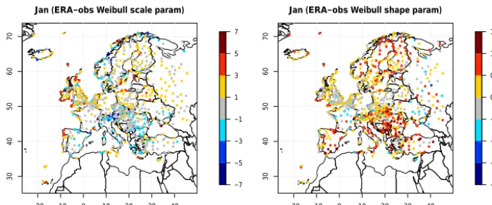
param-eters from the nearest ERA-Interim grid box. Figure 1 shows differences (ERA-Interim minus observations) between the scale and shape parameters for January across the European domain. The maps indicate generally good agreement for January, i.e. the values for the two parameters are
gener-ally within±1 of each other. Exceptions may be found in
some mountainous regions and around west-facing coasts but this is very dependent on the month (larger differences when wind speeds are stronger). The similarity of the two distribu-tions in terms of their scale and shape parameters indicates that bias adjustment could be achieved by replacing the ERA-Interim scale and shape parameters with those inferred from the HadISD stations.
Equation (3) of Tye et al. (2014) provides a means to
ad-just the original variableX into a variable X∗ having scale
and shape parametersα∗andβ∗by the following power-law
transfer function:
X∗=α∗
X α
β/β∗
. (3)
Where stations are available, α∗ and β∗ are those of the
−20 −10 0 10 20 30 40 30 40 50 60 70
Jan (ERA−obs Weibull scale param)
● ●●●● ● ●● ● ● ●●● ● ● ●● ●● ●● ● ● ● ● ● ● ● ● ● ●● ●●● ●●● ●● ●●●● ● ● ● ● ● ● ● ● ● ● ● ● ●● ●●●● ●●●● ● ● ● ● ●●●● ●●● ● ● ● ●●● ●● ● ● ● ●●●●● ● ● ● ●●●●● ●●●●●● ● ● ●●●●●● ●●●●●●●●●●●● ●●●●●●● ●● ● ● ●●●●●●●●● ● ●●● ● ● ● ● ●● ● ● ● ●●● ●●●● ●●●●●●●● ●●● ● ●●●●●●●● ●●●●●●● ● ● ●●●●●●●●●●● ●● ●● ● ● ●●●●●●●●● ● ● ● ● ●● ● ● ● ●● ● ● ●● ● ●● ●●● ●● ●●● ● ● ● ● ● ● ● ●●●●●● ● ●●●●●●●●●●●●● ● ● ● ● ●●●● ●●●●●●●● ●● ●● ●●●● ●●● ●●● ● ● ● ●●● ● ●●●●● ● ● ● ● ● ●●● ● ●● ● ●●●● ● ● ●●●●● ● ● ●● ● ● ● ●● ● ●●● ●●● ●● ● ●● ● ● ● ● ● ● ● ●● ●●●●● ● ● ● ●● ● ● ●●●●●●● ● ●●●●●●●●●● ● ●●●●●● ● ● ●● ● ● ● ● ●●● ● ●●●●●●● ●● ● ●●●●●●●●● ●●●●●● ● ●●● ●●●●● ●● ● ● ● ●●● ● ● ●●●● ●●●●●● ●●●● ● ● ●● ●●●● ● ●● ●●● ●● ● ● ● ●● ● ●●● ●● ●●●●●●●● ●● ●●●●●● ● ● ●● ● ● ● ●● ●●●●●● ● ● ●●●● ● ●●●●●●●●●● ●● ●● ●●● ●● ●● ● ●● ●●●●● ● ● ●● ●● ● ●● ● ● ● ● ● ● ● ● ● ● ● ● ●● ●●● ●●● ● ● ●●● ● ● ● ● ● ●● ●●● ●●●●●●●●●●● ●●●●●●●● ●●● ● ● ● ●● ● ● ● ● ● ● ● ● ● ● ● ● ●●● ● ● ● ● ●●●●● ● ●● ● ●●●● ●● ●● ●● ● ●● ● ● ● ● ● ● ● ● ● ● ● ● ● ● ● ● ● ● ● ● ● ● ● ● ● ● ● ● ●● ● ● ● ●● ●● ● ● ●● ● ●● ● ●● ● ● ● ●● ● ●●●●● ● ●● ● ● ● ●●● ● ●●●●● −7 −5 −3 −1 1 3 5 7
−20 −10 0 10 20 30 40
30
40
50
60
70
Jan (ERA−obs Weibull shape param)
● ●●●● ●● ●●● ●●● ● ● ●● ●● ●● ● ● ● ● ● ● ● ● ● ● ● ●●● ●●● ●● ●●●● ● ● ● ● ● ● ● ● ●● ● ● ●● ●●●● ●●●● ● ● ● ● ● ●●● ●●● ● ● ● ●●● ●● ● ● ● ●●●● ● ● ● ● ●●●●● ● ● ● ●● ● ● ● ●● ●●●● ●● ●●●●●●●●●● ●●●●●●● ● ● ● ● ●●●●●●●●●● ●●●● ● ●● ●● ● ● ●●●● ●●● ●●●●●●●●● ●● ● ● ●●●●●●●●●●●●●●● ●●●●●●●●●●●●● ●● ●● ● ●●●● ●●●●●● ● ● ● ● ●● ● ● ● ●● ● ● ●● ● ●● ● ●●●● ●●● ● ● ● ● ● ● ● ●●●●●● ● ●●●●●●●●●●●●● ●● ● ● ●● ●●●●●●●●●● ●● ●● ●●●● ●●●●● ●●●●●●●● ●●●●●●● ● ● ●●●● ● ●● ● ●●●● ● ● ● ●●●● ● ● ● ● ● ● ● ●● ● ●●● ●●● ●● ● ● ● ● ● ● ● ● ● ● ●● ●●●●● ● ● ● ●● ● ●●●●●●●● ● ●●●●●●●●●●● ● ●● ●●●● ● ● ● ● ● ● ● ● ●●● ● ●●●●●●●●● ● ●● ● ●●●●●●● ●●●●●● ● ●●● ●●●●● ●● ● ● ● ●●● ● ● ● ●●●● ●●●●●● ●●●● ● ● ●●●● ●●● ●● ●●● ●● ● ●● ●● ● ●●● ●●●● ●●●●●● ●●●●●●●●●●●●● ● ● ● ●● ●●●●●●● ●●●● ●●●●●●●●●●●●●● ●●● ● ● ●●●●● ●● ● ● ●● ●●●●● ● ● ● ● ●● ● ●● ● ● ●● ●● ● ● ● ● ● ● ●● ●●● ●●● ● ● ●● ● ● ● ●●● ●● ●●● ●●●●●●● ●●●●● ● ● ●● ●●● ●●● ● ● ● ●● ● ● ● ● ● ● ● ● ● ● ● ● ●● ● ● ●● ● ●●●●● ● ●●●●●● ●●●●●●● ●●● ●●●●● ● ● ● ● ● ● ● ● ● ● ● ● ● ● ● ● ● ● ● ● ● ● ●●●● ● ● ● ● ●● ● ● ●● ● ●● ● ●● ● ● ● ●● ● ●●●●● ● ●● ●● ● ●● ● ● ●●●●● −1.75 −1.25 −0.75 −0.25 0.25 0.75 1.25 1.75
Figure 1.Differences in scale and shape parameters of the Weibull distribution between ERA-Interim and HadISD station observations for wind speed at 10 m. Based on all 6-hourly data for January for 1981–2010.
and a few sites in mountainous regions (see the full set of distributional fits on the ftp site). Some observed distribu-tions are a little erratic due to some years in the observed data having wind speeds rounded to integer values. Similarly to Fig. 1, but for bias-adjusted ERA-Interim minus observa-tions, Fig. 4 shows differences between the scale and shape parameters for January. Almost all stations across Europe ex-hibit similar shape and scale parameters between the stations and adjusted ERA-Interim. However, a few stations in coastal areas and at high-elevation mountain locations still show dif-ferences in parameters. The fit is not perfect as the estimation of the shape and scale parameters for the ERA-Interim grid boxes from HadISD is influenced by the station distribution. In addition, the number of stations in some parts of Europe is less dense and so involves greater extrapolation from stations more distant from the grid boxes.
4.2 Surface air temperature, dewpoint temperature, and relative humidity
Like wind speed, both surface air temperature and dewpoint temperature are produced from ERA-Interim every 6 h. Un-like 10 m wind, both these variables have a strong diurnal cycle, which is generally slightly stronger in the summer. A normal distribution was fitted using daily averages of tem-perature, taking the average of the four 6 h data for each day. E-OBS is the dataset on which ERA-Interim is to be adjusted for air temperature. For dewpoint we use HadISD, but we combine this with air temperatures from HadISD to calculate dewpoint depression (DPD), the difference between air and dewpoint temperature. To calculate DPD, we need to pair off air and dewpoint temperature measurements taken every 6 h.
DPD will always be ≥0, so we use a Weibull distribution
to ensure that any bias adjustments always produce a DPD
that is≥0. Means and standard deviations of the daily
aver-age of air temperature are calculated for each month of the
year for each 0.5◦grid cell of ERA-Interim coincident with
the E-OBS grid box. The distributional parameters for DPD
are interpolated as for wind speed; then, based on air tem-perature, a dewpoint temperature can be calculated. Data are normalized as in Eq. (4) and transformed back by Eq. (5) for air temperature.
TERA0 =TERA−TERA
σERA
, (4)
T∗=TERA0 σobs+Tobs, (5)
where T0 is the normalized ERA-Interim temperature
anomaly,T∗is the bias-adjusted ERA-Interim temperature,
T is the mean temperature, andσ is the standard deviation.
Bias adjustment works by transforming the normalized ERA-Interim grid-box time series back to air temperatures using the means and standard deviations from E-OBS and interpo-lations from station data in HadISD for DPD. Once daily av-erages are adjusted, the difference between the original ERA-Interim daily mean and the adjusted daily mean is added to each of the four 6 h temperatures within each day. Therefore, no alteration is made to each diurnal cycle of air tempera-ture or DPD. This yields the final set of bias-adjusted 6 h surface air and dewpoint temperatures (the latter calculated from DPD) consistent with one another.
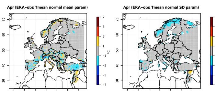
Figure 5 shows the differences in the mean and standard deviation for air temperature for April as an example. There is good agreement between estimates for ERA-Interim and those calculated from E-OBS. As these are both gridded
datasets, the maps shown are fully coloured for each 0.5◦
grid box. Differences in Fig. 5 are likely related to
eleva-tional differences in the 0.5◦grid boxes between E-OBS and
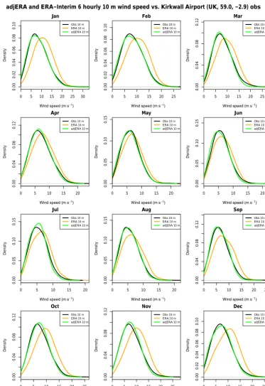
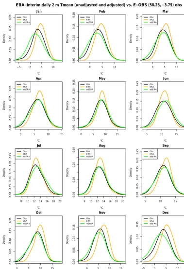
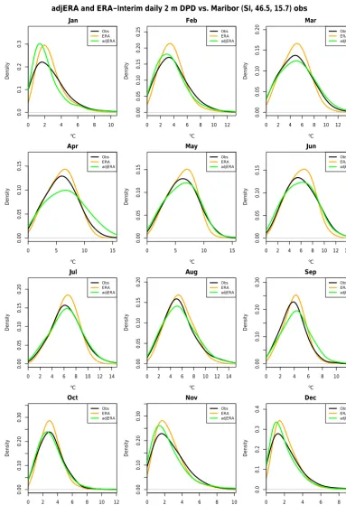
ERA-Interim. The significance of this is discussed more in Sect. 4.5 when our adjusted ERA-Interim and the WFDEI datasets are separately compared with E-OBS. Figures 6 and 7 exhibit the distributional fits of the E-OBS, original ERA-Interim, and bias-adjusted ERA-Interim for the 12 cal-endar months for the nearest land grid boxes that approxi-mate the locations of Kirkwall and Maribor used for wind
0 5 10 15 20 25 30
0.00
0.02
0.04
0.06
0.08
0.10
Jan
Wind speed (m s- 1)
Density
Obs 10 m ERA 10 m adjERA 10 m
0 5 10 15 20 25
0.00
0.02
0.04
0.06
0.08
0.10
Feb
Wind speed (m s- 1)
Density
Obs 10 m ERA 10 m adjERA 10 m
0 5 10 15 20 25
0.00
0.04
0.08
0.12
Mar
Wind speed (m s- 1)
Density
Obs 10 m ERA 10 m adjERA 10 m
0 5 10 15 20
0.00
0.04
0.08
0.12
Apr
Wind speed (m s- 1)
Density
Obs 10 m ERA 10 m adjERA 10 m
0 5 10 15 20
0.00
0.05
0.10
0.15
May
Wind speed (m s- 1)
Density
Obs 10 m ERA 10 m adjERA 10 m
0 5 10 15 20
0.00
0.05
0.10
0.15
Jun
Wind speed (m s- 1)
Density
Obs 10 m ERA 10 m adjERA 10 m
0 5 10 15 20
0.00
0.05
0.10
0.15
Jul
Wind speed (m s- 1)
Density
Obs 10 m ERA 10 m adjERA 10 m
0 5 10 15 20
0.00
0.05
0.10
0.15
Aug
Wind speed (m s- 1)
Density
Obs 10 m ERA 10 m adjERA 10 m
0 5 10 15 20 25
0.00
0.04
0.08
0.12
Sep
Wind speed (m s- 1)
Density
Obs 10 m ERA 10 m adjERA 10 m
0 5 10 15 20 25
0.00
0.04
0.08
0.12
Oct
Wind speed (m s- 1)
Density
Obs 10 m ERA 10 m adjERA 10 m
0 5 10 15 20 25
0.00
0.04
0.08
0.12
Nov
Wind speed (m s- 1)
Density
Obs 10 m ERA 10 m adjERA 10 m
0 5 10 15 20 25
0.00
0.02
0.04
0.06
0.08
0.10
Dec
Wind speed (m s- 1)
Density
Obs 10 m ERA 10 m adjERA 10 m
adjERA and ERA−Interim 6 hourly 10 m wind speed vs. Kirkwall Airport (UK, 59.0, −2.9) obs
Figure 2. Comparison of statistical distributions of wind speed at 10 m for Kirkwall, Scotland, for observations (black), ERA-Interim (orange), and bias-adjusted ERA-Interim (green), based on all 6-hourly data for the 1981–2010 period.
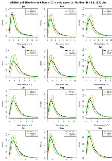
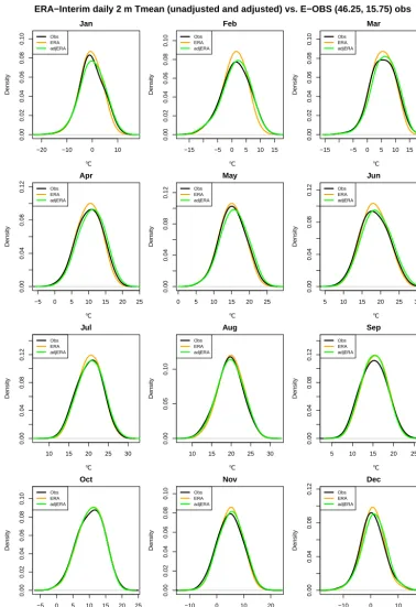
is located. Kirkwall is on the Orkney Islands, so the near-est grid box within E-OBS is located further south in north-ern Scotland. The distributional fits for the Maribor grid box were good for ERA-Interim, and bias adjustment brings
0 2 4 6 8 10 12
0.0
0.1
0.2
0.3
0.4
Jan
Density
Obs 10 m ERA 10 m adjERA 10 m
0 2 4 6 8 10 12 14
0.0
0.1
0.2
0.3
0.4
Feb
Density
Obs 10 m ERA 10 m adjERA 10 m
0 2 4 6 8 10 12
0.0
0.1
0.2
0.3
0.4
Mar
Density
Obs 10 m ERA 10 m adjERA 10 m
0 2 4 6 8 10
0.0
0.1
0.2
0.3
0.4
Apr
Density
Obs 10 m ERA 10 m adjERA 10 m
0 2 4 6 8 10 12
0.0
0.1
0.2
0.3
0.4
May
Density
Obs 10 m ERA 10 m adjERA 10 m
0 2 4 6 8 10
0.0
0.1
0.2
0.3
0.4
0.5
Jun
Density
Obs 10 m ERA 10 m adjERA 10 m
0 2 4 6 8
0.0
0.1
0.2
0.3
0.4
0.5
Jul
Density
Obs 10 m ERA 10 m adjERA 10 m
0 2 4 6 8 10
0.0
0.1
0.2
0.3
0.4
0.5
Aug
Density
Obs 10 m ERA 10 m adjERA 10 m
0 2 4 6 8 10
0.0
0.1
0.2
0.3
0.4
0.5
Sep
Density
Obs 10 m ERA 10 m adjERA 10 m
0 2 4 6 8 10
0.0
0.1
0.2
0.3
0.4
Oct
Density
Obs 10 m ERA 10 m adjERA 10 m
0 2 4 6 8 10 12
0.0
0.1
0.2
0.3
0.4
Nov
Density
Obs 10 m ERA 10 m adjERA 10 m
0 2 4 6 8 10
0.0
0.1
0.2
0.3
Dec
Density
Obs 10 m ERA 10 m adjERA 10 m
adjERA and ERA−Interim 6 hourly 10 m wind speed vs. Maribor (SI, 46.5, 15.7) obs
Wind speed (m s- 1) Wind speed (m s- 1) Wind speed (m s- 1)
Wind speed (m s- 1) Wind speed (m s- 1) Wind speed (m s- 1)
Wind speed (m s- 1) Wind speed (m s- 1) Wind speed (m s- 1)
Wind speed (m s- 1) Wind speed (m s- 1) Wind speed (m s- 1)
Figure 3.Comparison of statistical distributions of wind speed at 10 m for Maribor, Slovenia, for observations (black), ERA-Interim (orange), and bias-adjusted ERA-Interim (green), based on all 6-hourly data for the 1981–2010 period.
Kirkwall example and also most of the northern and eastern Europe comparisons illustrate an issue with approximating daily air temperature by a normal distribution for winter. For
−20 −10 0 10 20 30 40 30 40 50 60 70
Jan (adjERA−obs Weibull scale param)
● ● ●●● ●● ●● ● ● ●● ● ● ●●● ● ●● ● ● ● ● ● ● ●● ● ● ● ●●● ●●● ●● ●●●● ● ● ● ● ● ● ● ● ● ● ● ● ● ● ●●●● ●●●● ● ● ● ● ● ●● ● ●●● ● ● ● ●●●●●● ● ● ● ●●● ● ● ● ● ●● ● ●● ● ● ● ●●●● ● ●● ● ● ●●● ● ●●● ● ● ●● ● ●● ●●●●●●● ● ● ● ● ●●●●●●●●●● ●●●● ● ●● ●● ● ● ●●●● ●●●●● ● ●●●●●● ●● ● ● ●●●●●●●●●● ●●●●● ● ●●●●●●●●●●●● ●● ● ● ● ● ●●●● ●● ● ●● ● ● ● ●● ● ●● ● ●●● ● ●●● ● ● ● ● ● ● ● ●●●●●● ●●●●●●●●●●●●● ●● ● ● ●●●● ●●●●●●●● ● ● ●● ●●●● ●●● ●●● ● ● ● ●● ●● ● ●● ● ● ● ● ● ● ● ● ●●●●● ● ●● ●● ● ● ●●●●● ● ● ● ● ● ● ● ●● ●●● ● ●● ● ● ● ● ● ● ● ● ● ● ●● ●●●●● ● ● ● ●● ● ● ●●●●●●● ● ●●●●●●●●●●● ● ●●●●● ● ● ● ●● ● ● ● ● ●●● ● ●●●●●●● ●● ● ●●●●●●●●● ●●●●●● ● ●●●●●● ● ● ●●● ●● ●●● ● ● ● ● ●●●● ●●● ● ●●● ● ● ●●● ●● ●●● ●● ●●● ●● ● ● ● ● ● ● ●●● ●● ●●●●●●● ●● ●●●●●● ●● ●● ● ● ● ●● ●●● ●●● ● ● ●●●● ● ●●●●●●●●●● ●● ● ● ●●●●● ● ● ● ●●● ●●●● ● ● ● ● ●● ● ●● ● ● ● ● ● ● ● ● ● ● ● ● ● ● ●●● ●●● ● ● ●● ● ● ● ● ● ●●● ●● ● ●● ● ●● ●● ● ● ● ● ● ● ●● ●●● ●● ● ● ●● ● ● ● ● ● ● ● ● ● ● ●● ● ● ● ● ● ● ●● ● ● ●● ●●●● ●● ●● ●● ●● ● ●● ● ●● ● ● ● ● ● ● ● ● ● ●● ● ● ● ● ● ● ● ● ● ● ● ●● ● ● ● ● ● ● ● ● ●● ● ●● ● ● ● ● ● ● ●● ● ●●●●● ● ● ● ● ● ● −7 −5 −3 −1 1 3 5 7
−20 −10 0 10 20 30 40
30
40
50
60
70
Jan (adjERA−obs Weibull shape param)
● ● ●●● ●● ●● ● ● ●● ● ● ●●● ● ●● ● ● ● ● ● ● ● ● ● ●● ●●● ●●● ●● ●●●● ● ● ● ● ● ● ● ● ● ● ● ● ● ● ●●●● ●●●● ● ● ● ● ●●● ● ●●● ● ● ● ●●●●●● ● ● ●●● ● ● ● ● ● ●● ● ●● ● ● ●●●●● ● ●● ● ● ●●● ● ●●● ● ● ●● ● ●● ●●● ●●●● ● ● ● ● ●●●●●●●●●● ●●●● ● ●● ●● ● ● ●●●● ●●●●● ● ●●●●●● ●● ● ● ●●●●●●●●●●●●●●● ● ●●●●●●●●●●●● ●● ● ● ● ● ●●●● ●● ● ●● ● ● ● ●● ● ●● ● ●●●● ●●● ● ● ● ● ● ● ● ●●●●●● ●●●●●●●●●●●●● ●● ● ● ●●●●●●●●●●●● ● ● ●● ●●●● ●●● ●●● ● ● ● ●●●● ● ●● ● ● ● ● ● ● ● ● ●● ● ● ● ● ●● ●● ● ● ●●●●● ● ● ● ● ● ● ● ●● ●●● ● ●● ● ● ● ● ● ● ● ● ● ● ●● ●●●●● ● ● ● ●● ● ● ●●●●●●● ● ●●●●●●●●●●● ● ●●●●● ● ● ● ●● ● ● ● ● ●●● ● ●●●●●●●●● ● ● ●●●●●●●●● ●●●●●● ● ●●●●●● ● ● ●●● ●● ●●● ● ● ● ●● ●●●● ●●● ● ●●●● ● ● ●●●● ●●● ●● ●●● ●● ● ●● ●● ● ●●● ●● ●●●●●●● ●●● ●●●●●● ●● ●● ● ● ● ●● ●●● ●●●● ● ● ●●●●● ● ●●●●●●●●●● ● ● ● ● ● ●●●●● ● ● ● ● ●● ●● ● ●● ● ● ● ● ●● ● ●● ● ● ● ● ● ● ● ● ● ● ● ● ● ● ●●● ●●● ● ● ●● ● ● ●●● ●●● ●● ● ●● ● ●● ●● ● ● ● ● ● ● ●● ●●● ●● ● ● ●● ● ● ● ● ● ● ● ● ● ● ●● ● ● ● ● ● ● ●● ● ● ●● ●●●● ●● ●●●● ●● ● ●● ● ●● ● ● ● ● ● ● ● ● ● ●● ● ● ● ● ● ● ● ● ● ● ● ●● ● ● ● ● ● ● ● ● ●● ● ●● ● ●● ● ● ● ●● ● ●●●●● ● ● ● ● ● ● −1.75 −1.25 −0.75 −0.25 0.25 0.75 1.25 1.75
Figure 4.Differences in scale and shape parameters of the Weibull distribution between bias-adjusted ERA-Interim and HadISD station observations for wind speed at 10 m. Based on all 6-hourly data for January for 1981–2010.
−20 −10 0 10 20 30 40
30 40 50 60 70 −7 −5 −3 −1 1 3 5 7
−20 −10 0 10 20 30 40
30
40
50
60
70
Apr (ERA−obs Tmean normal mean param)
−20 −10 0 10 20 30 40
30 40 50 60 70 −3.5 −2.5 −1.5 −0.5 0.5 1.5 2.5 3.5
o C
−20 −10 0 10 20 30 40
30
40
50
60
70
Apr (ERA−obs Tmean normal SD param)
oC
Figure 5.Differences in means and standard deviations (SDs) between ERA-Interim and E-OBS for mean surface air temperature (Tmean). Based on daily data for April for 1981–2010.
daily timescale. Horton et al. (2001) experimented with an alternate distribution (an inverted gamma distribution), but this adds an additional parameter to any bias-adjustment ap-proach and fitting requires an interactive procedure. Figure 8 shows the differences between the means and standard de-viations, but this time after adjustment, to allow comparison with Fig. 5.
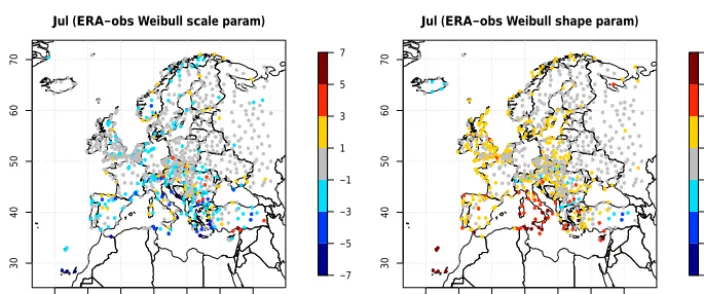
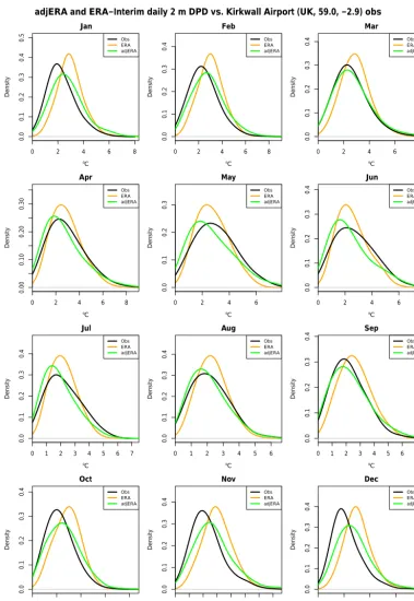
Figure 9 shows the differences in the Weibull distribu-tion parameter plots for DPD for July. There is good agree-ment between estimates from ERA-Interim and those cal-culated from HadISD using DPD. This plot shows the sta-tion locasta-tions in a similar fashion to that for wind speed in Fig. 1. Figures 10 and 11 show the distributional fits of the HadISD, original Interim, and bias-adjusted ERA-Interim for DPD for the 12 calendar months for the loca-tions of Kirkwall and Maribor. Both examples of distribu-tional plots adjust ERA-Interim slightly, but the original fits were quite good to start with. As with wind speed, the DPD
distributions are curtailed for values<0. Similarly to Fig. 9,
Fig. 12 shows the differences between the Weibull distribu-tion parameters for DPD but after adjustment.
With the adjustments for dewpoint temperature using DPD, it is a simple task to then calculate relative humidity (RH) using the adjusted air temperature. Performing the bias adjustment this way, we are assured that all RH values are between 0 and 100 %.
4.3 Daily precipitation totals
The same process was then used for daily precipitation to-tals but using a gamma distribution, which has been found to perform well in many studies (e.g. Wilks, 1995).
F(x;α, β)=
x
β
α−1exp
−x
β
β0(α) (6)
Gamma distributions have two parameters, shape (α) and
scale (β), and were fit to the daily precipitation totals for
each month for ERA-Interim and for E-OBS. In Eq. (6),
we show the probability density function where 0 is the
ignor-−5 0 5 10
0.00
0.05
0.10
0.15
0.20
Jan
oC
Density
Obs ERA adjERA
0 5 10
0.00
0.05
0.10
0.15
0.20
Feb
oC
Density
Obs ERA adjERA
0 5 10 15
0.00
0.05
0.10
0.15
0.20
Mar
oC
Density
Obs ERA adjERA
0 5 10 15
0.00
0.05
0.10
0.15
0.20
Apr
oC
Density
Obs ERA adjERA
0 5 10 15
0.00
0.05
0.10
0.15
0.20
0.25
May
oC
Density
Obs ERA adjERA
5 10 15
0.00
0.05
0.10
0.15
0.20
0.25
Jun
oC
Density
Obs ERA adjERA
8 10 12 14 16 18 20
0.00
0.05
0.10
0.15
0.20
0.25
Jul
oC
Density
Obs ERA adjERA
8 10 12 14 16 18 20
0.00
0.10
0.20
0.30
Aug
oC
Density
Obs ERA adjERA
5 10 15
0.00
0.05
0.10
0.15
0.20
0.25
Sep
oC
Density
Obs ERA adjERA
0 5 10 15
0.00
0.05
0.10
0.15
0.20
Oct
oC
Density
Obs ERA adjERA
0 5 10 15
0.00
0.05
0.10
0.15
Nov
oC
Density
Obs ERA adjERA
−5 0 5 10 15
0.00
0.05
0.10
0.15
Dec
oC
Density
Obs ERA adjERA
ERA−Interim daily 2 m Tmean (unadjusted and adjusted) vs. E−OBS (58.25, −3.75) obs
Figure 6.Comparison of statistical distributions of surface air temperature for northern Scotland (58.25◦N, 3.75◦W), for observations (black), ERA-Interim (orange), and bias-adjusted ERA-Interim (green), based on daily data for the 1981–2010 period.
ing all precipitation values below a fixed low daily precipita-tion threshold over the whole domain. Thresholds of 0.4, 0.6, 0.8, and 1.0 mm were experimented with and best fits were achieved with 1.0 mm. This implies that the gamma
−20 −10 0 10
0.00
0.02
0.04
0.06
0.08
0.10
Jan
Density
Obs ERA adjERA
−15 −5 0 5 10 15
0.00
0.02
0.04
0.06
0.08
0.10
Feb
Density
Obs ERA adjERA
−15 −5 0 5 10 15 20
0.00
0.02
0.04
0.06
0.08
0.10
Mar
Density
Obs ERA adjERA
−5 0 5 10 15 20 25
0.00
0.04
0.08
0.12
Apr
Density
Obs ERA adjERA
0 5 10 15 20 25
0.00
0.04
0.08
0.12
May
Density
Obs ERA adjERA
5 10 15 20 25 30
0.00
0.04
0.08
0.12
Jun
Density
Obs ERA adjERA
10 15 20 25 30
0.00
0.04
0.08
0.12
Jul
Density
Obs ERA adjERA
10 15 20 25 30
0.00
0.05
0.10
Aug
Density
Obs ERA adjERA
5 10 15 20 25
0.00
0.04
0.08
0.12
Sep
Density
Obs ERA adjERA
−5 0 5 10 15 20 25
0.00
0.02
0.04
0.06
0.08
0.10
Oct
Density
Obs ERA adjERA
−10 0 10 20
0.00
0.02
0.04
0.06
0.08
0.10
Nov
Density
Obs ERA adjERA
−10 0 10 20
0.00
0.04
0.08
0.12
Dec
Density
Obs ERA adjERA
ERA−Interim daily 2 m Tmean (unadjusted and adjusted) vs. E−OBS (46.25, 15.75) obs
oC oC oC
oC oC oC
oC oC oC
oC oC oC
Figure 7.Comparison of statistical distributions of surface air temperature for the Maribor grid box (46.25◦N, 15.75◦E), for observations (black), ERA-Interim (orange), and bias-adjusted ERA-Interim (green), based on daily data for the 1981–2010 period.
essence areal averages, more than would be the case for a station rain gauge series. In the adjusted ERA-Interim all pre-cipitation amounts below the threshold are set to zero, further improving the agreement between E-OBS and ERA-Interim
−20 −10 0 10 20 30 40 30 40 50 60 70 −7 −5 −3 −1 1 3 5 7
−20 −10 0 10 20 30 40
30
40
50
60
70
Apr (adjERA−obs Tmean normal mean param)
−20 −10 0 10 20 30 40
30 40 50 60 70 −3.5 −2.5 −1.5 −0.5 0.5 1.5 2.5 3.5
−20 −10 0 10 20 30 40
30
40
50
60
70
Apr (adjERA−obs Tmean normal SD param)
oC oC
Figure 8.Differences in means and standard deviations (SDs) between bias-adjusted ERA-Interim and E-OBS for mean surface air temper-ature (Tmean). Based on all data for April for 1981–2010.
−20 −10 0 10 20 30 40
30
40
50
60
70
Jul (ERA−obs Weibull scale param)
● ●●●● ● ●●● ● ● ●● ● ●●● ●● ●● ● ● ● ● ● ● ● ● ● ● ● ● ●●●●● ●● ●●●● ● ● ● ● ● ● ● ● ● ● ● ● ●●●●●● ●●●● ● ● ● ● ● ●● ● ●●● ● ● ● ●●●●●● ● ● ● ● ●●● ● ●●●●●●●● ● ● ●●● ● ● ● ●● ●●● ●● ● ●●● ● ●● ● ●● ●●● ●●●● ● ● ● ● ●●●●●●●●● ● ●●●●● ●● ● ●●● ●●●● ●●●●●●● ● ● ●● ●● ● ● ●●●●●●●●●●●●●● ● ●●●●●●●●●● ● ●● ● ● ● ● ●●●● ●●●● ● ● ● ● ● ● ● ● ● ● ●● ● ● ●● ● ●● ●● ●● ●● ● ● ● ●● ● ● ● ● ●●●●●● ●●●● ●●●●● ● ● ● ● ● ●● ● ● ●●●● ●●●●●●●● ● ●●● ●●●● ●● ●●● ● ● ● ● ●●●● ● ●●● ●● ●● ●● ●●●● ● ●● ● ●●●● ● ● ●●●●●● ● ● ●●● ● ● ● ●● ●●●● ● ●● ●● ● ● ● ● ● ● ● ● ● ● ●● ●●●●● ● ● ● ●● ● ● ●●●●●●● ● ●●●●●●●●●●●● ● ●●●●●● ● ● ● ●● ● ● ● ● ● ●●●●●●●●●●● ●● ● ●● ● ●●●●●●● ●●●●●● ● ● ●● ●●●●●●● ● ● ●●● ● ● ●●●●●●● ● ●● ●●●●● ●●● ● ● ●● ● ● ● ●●●●●●● ●● ●●● ● ● ●● ● ● ● ● ● ●●● ● ●●●● ●●●●●● ●●●●●●●●●●●●●●●● ●●● ● ● ● ● ●●●●●●● ● ● ●●●●●●● ●●●●●●●●●●● ●●●● ●● ●●●●●● ● ●● ● ● ●●●●●●● ● ● ●● ● ● ● ●● ● ● ●● ●● ● ● ● ● ● ●● ● ●● ● ● ● ●●● ● ●●● ● ●●●● ●● ●●● ●●●●● ● ● ●●● ● ● ●●●● ● ●● ●●● ●●● ● ● ● ● ● ● ● ● ● ● ● ●● ● ● ● ● ● ● ● ●●●● ● ● ● ● ● ● ●●● ●● ●● ● ● ●● ● ● ●● ● ●● ● ● ● ● ● ● ● ● ● ● ●● ● ●●●●● ●●● ● ●● ● ● ● ● ● ●● ● ● ● ● ●●● ● ●● ● ●● ● ● ●●●● ●● ●●●● ● ● ● ●● ● ●● ●● ● ●● ● ●● ● ● ● ● ● ●● ● ● ● ●●●●● ● ●●●● ●● ● ● ● ● ● ● ● ●●●●● −7 −5 −3 −1 1 3 5 7
−20 −10 0 10 20 30 40
30
40
50
60
70
Jul (ERA−obs Weibull shape param)
● ● ●●● ● ●●●● ● ●● ● ●●● ●● ●● ● ● ● ● ● ● ●● ● ●● ● ●●●●● ●● ●●●● ● ● ● ● ● ● ● ● ● ● ● ● ● ● ●●● ● ●●●● ● ● ● ● ● ●● ● ●●● ● ● ● ●●●●● ● ● ● ● ● ●●● ● ●●●●● ● ●● ● ● ● ●● ● ● ● ●● ● ● ●●● ● ●●● ● ●● ●●● ●●●●●●● ● ● ● ● ●●●●●●●●● ● ●●●●● ● ● ● ●●● ●●●● ●●●●●●● ●● ●● ●●● ● ●●●●●●●●●●●●●● ● ●●●●●●●●●● ● ●● ● ● ●●●●●●●●●●●● ● ● ● ●● ● ● ● ●● ● ● ●● ● ●● ●● ● ● ●●●● ● ● ● ● ● ● ● ●●●●●● ●●●●●●●●●●● ● ● ● ●● ● ● ●●●● ●●●●●●●● ● ●●● ●●●● ●● ●●● ● ● ● ●●●● ●●● ● ●●● ● ●● ● ●●●● ● ● ● ● ●●●●● ● ●● ●●●● ● ● ●●● ● ● ● ●● ●●●● ●●● ●● ● ●● ● ● ● ● ● ● ● ●● ●●●●● ● ● ● ●● ● ● ●●●●●●● ● ●●●●●●●●●●●● ● ●● ●●●● ● ● ● ●● ●● ● ● ● ●● ●● ●●●●●●● ●● ●●● ● ●●●●●●● ●●●●●●●● ●●● ●●●● ●●●● ●● ● ● ● ●●●●● ●● ● ●● ●● ●●● ●●● ● ● ●●● ● ● ●●●●●●● ●● ●●● ● ● ●● ●● ● ●● ●●● ● ●● ● ●●●●● ●● ●●●●●●●●●●●●●●●● ●●● ● ● ● ● ●●●●●●● ●● ●●●●●●●●●●●●●●● ● ● ● ●●●● ●● ●●●●● ● ●●●●●●●●● ● ● ●●● ● ● ● ● ● ●● ● ● ●● ●● ● ● ● ● ● ●● ● ●● ● ● ● ●●● ● ●●● ● ● ● ●● ●● ●●● ●●●● ●● ● ●●● ● ● ●●●● ● ●● ●●● ●●● ● ● ● ● ● ● ● ● ● ● ● ●● ● ● ● ● ● ● ● ●● ● ● ● ● ● ● ● ● ●●● ●● ●● ● ● ●●●●● ●● ●● ● ● ● ● ● ● ● ● ● ● ●● ● ● ● ● ● ● ●●● ● ●● ● ● ● ● ● ●● ● ● ● ● ●●● ● ● ● ● ● ●●●● ●● ●●● ● ● ● ● ● ● ● ● ● ● ●● ●● ● ●●● ●● ● ●● ● ● ●● ● ● ● ●●●●● ● ● ● ● ● ●● ● ● ● ● ● ● ● ●●●●● −3.5 −2.5 −1.5 −0.5 0.5 1.5 2.5 3.5
Figure 9.Differences in means and standard deviations (SDs) between ERA-Interim and HadISD for dewpoint temperature (◦C). Based on daily data for July for 1981–2010.
transformed ERA-Interim precipitation total with the scale and shape parameters from the E-OBS dataset.
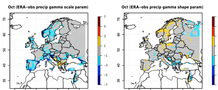
Figure 13 shows the differences in the scale and shape parameters of the gamma distribution for October, by way of example. There is good agreement between estimates for ERA-Interim and those calculated from E-OBS. As these are both gridded datasets, the maps shown are fully coloured for
each 0.5◦grid box. Of the 4520 possibilities, Figs. 14 and 15
exhibit the distributional fits of the E-OBS, original ERA-Interim, and bias-adjusted ERA-Interim datasets for the 12 calendar months for the nearest land grid boxes that approx-imate the locations of Kirkwall and Maribor. The fits for the northern Scotland grid box are considerably better than for Maribor, where the distributional fits are slightly worse for April–August. Here only two locations are shown as exam-ples: the full set of results for the 4520 grid-box comparisons can be viewed at the ftp site. The complete set uses common scaling, which may be inappropriate in drier parts of Europe and the fits (shown in the two examples in Figs. 14 and 15 are smoothed representations of the distributions curtailed at zero rainfall). Although the gamma distribution is widely
used for rainfall data, it is not ideal in all climates and across all seasons in Europe. Problems arise when there are too few rainfall days within dry seasons (the southern Mediterranean and the Middle East during summer). Similarly to Fig. 13, Fig. 16 shows the differences between the scale and shape parameters after adjustment.
4.4 Surface solar irradiance
For the sake of simplicity, the adjustment was performed on the daily mean of irradiance. Three methods have been in-vestigated: ratio, affine, and quantile mapping. Each method
may be applied to the clearness indicesKtas well. The
pos-sible improvement in bias delivered by each method was as-sessed by comparing the original ERA-Interim estimates and the bias-adjusted ERA-Interim with measurements from the 55 WRDC stations. The method “ratio” consists of
comput-ing the means of HC3v5 IHC3v5 and ERA-Interim IERA for
the calibration period of 2005–2014, then computing the
ra-tio of these means (IHC3v5/ IERA), and eventually
func-0 2 4 6 8
0.0
0.1
0.2
0.3
0.4
0.5
Jan
Density
Obs ERA adjERA
0 2 4 6 8
0.0
0.1
0.2
0.3
0.4
Feb
Density
Obs ERA adjERA
0 2 4 6 8
0.0
0.1
0.2
0.3
0.4
Mar
Density
Obs ERA adjERA
0 2 4 6 8
0.00
0.10
0.20
0.30
Apr
Density
Obs ERA adjERA
0 2 4 6
0.0
0.1
0.2
0.3
May
Density
Obs ERA adjERA
0 2 4 6
0.0
0.1
0.2
0.3
0.4
Jun
Density
Obs ERA adjERA
0 1 2 3 4 5 6 7
0.0
0.1
0.2
0.3
0.4
Jul
Density
Obs ERA adjERA
0 1 2 3 4 5 6
0.0
0.1
0.2
0.3
0.4
Aug
Density
Obs ERA adjERA
0 1 2 3 4 5 6 7
0.0
0.1
0.2
0.3
0.4
Sep
Density
Obs ERA adjERA
0 2 4 6 8
0.0
0.1
0.2
0.3
0.4
Oct
Density
Obs ERA adjERA
0 1 2 3 4 5 6 7
0.0
0.1
0.2
0.3
0.4
Nov
Density
Obs ERA adjERA
0 2 4 6 8
0.0
0.1
0.2
0.3
0.4
Dec
Density
Obs ERA adjERA
adjERA and ERA−Interim daily 2 m DPD vs. Kirkwall Airport (UK, 59.0, −2.9) obs
oC oC oC
oC oC oC
oC oC oC
oC oC oC
Figure 10.Comparison of statistical distributions of DPD for Kirkwall, for HadISD observations (black), ERA-Interim (orange), and bias-adjusted ERA-Interim (green), based on daily data for the 1981–2010 period.
tion between HC3v5 and ERA for the calibration period and then applying this function to the ERA-Interim estimates. The method “quantile mapping” was used here (applied to the clearness index) and consists of adjusting the cumulative
0 2 4 6 8 10
0.0
0.1
0.2
0.3
Jan
Density
Obs ERA adjERA
0 2 4 6 8 10 12
0.00
0.05
0.10
0.15
0.20
0.25
Feb
Density
Obs ERA adjERA
0 2 4 6 8 10 12 14
0.00
0.05
0.10
0.15
0.20
Mar
Density
Obs ERA adjERA
0 5 10 15
0.00
0.05
0.10
0.15
Apr
Density
Obs ERA adjERA
0 5 10 15
0.00
0.05
0.10
0.15
May
Density
Obs ERA adjERA
0 2 4 6 8 10 12 14
0.00
0.05
0.10
0.15
Jun
Density
Obs ERA adjERA
0 2 4 6 8 10 12 14
0.00
0.05
0.10
0.15
0.20
Jul
Density
Obs ERA adjERA
0 2 4 6 8 10 12 14
0.00
0.05
0.10
0.15
0.20
Aug
Density
Obs ERA adjERA
0 2 4 6 8 10 12
0.00
0.10
0.20
0.30
Sep
Density
Obs ERA adjERA
0 2 4 6 8 10 12
0.00
0.10
0.20
0.30
Oct
Density
Obs ERA adjERA
0 2 4 6 8 10
0.00
0.10
0.20
0.30
Nov
Density
Obs ERA adjERA
0 2 4 6 8
0.0
0.1
0.2
0.3
0.4
Dec
Density
Obs ERA adjERA
adjERA and ERA−Interim daily 2 m DPD vs. Maribor (SI, 46.5, 15.7) obs
oC oC oC
oC oC oC
oC oC oC
oC oC oC
Figure 11.Comparison of statistical distributions of DPD for Maribor, for HadISD observations (black), ERA-Interim (orange), and bias-adjusted ERA-Interim (green), based on daily data for the 1981–2010 period.
Figure 17 exhibits the bias for ERA-Interim vs. ground observations of daily mean of solar irradiance for the 55 sta-tions. Downward triangles mean a negative bias of more than
−5 W m−2, upward triangles mean a positive bias greater
than 5 W m−2, and circles mean an absolute value of the bias
−20 −10 0 10 20 30 40 30 40 50 60 70
Jul (adjERA−obs Weibull scale param)
● ●●●● ● ●● ● ● ● ●● ● ● ●●● ● ●●● ● ● ● ● ● ● ● ● ● ● ● ●●●●● ● ● ●●●● ● ● ● ● ● ● ● ● ● ● ● ● ●●●●● ● ●●●● ● ● ● ● ●●● ● ●●● ● ● ● ● ●●● ● ● ● ● ● ● ●●● ● ● ● ● ● ● ●●● ● ● ●●●●● ● ●● ● ● ●●● ● ●●● ● ●● ● ●● ●●● ●●●● ● ● ● ● ●●●●●●● ●● ● ●●●●● ●● ●● ● ● ●●●● ●●●●● ● ●●●●● ●● ● ● ●●●●●●●●●●●●●● ● ●●●●●●●●●● ● ●● ● ● ● ● ●●●● ● ● ● ●● ● ● ●● ● ● ● ● ● ●● ● ● ●● ● ●● ●● ●● ●●● ●●●● ● ● ● ● ●●●●●● ●●●●●●●●●●● ● ● ●●● ● ● ●●●● ●●●●●●●● ● ● ●● ●●●● ●●● ●●● ● ● ● ●● ●● ● ● ● ●● ●● ● ● ●●●●● ● ●● ● ●● ●● ● ● ●● ●●●● ● ● ● ●● ● ● ● ●● ● ●●● ● ● ● ●● ● ● ● ● ● ● ● ● ● ● ●● ●●●●● ● ● ● ●● ● ● ●●●●●●● ● ●●●●●●●●●●●● ● ●●●●● ● ● ● ● ●● ● ● ● ● ● ●●●●●●●●●●● ●● ● ●● ●●●●●●●● ●●●●●●● ● ● ● ●●● ●●● ● ● ● ●●● ●● ●●●●●●● ● ●● ●●●●● ●●● ● ●●● ● ● ● ●●●● ●●● ●● ●●● ●●●● ● ● ● ●● ●●●● ●● ●●●●●●●● ●●●●●●●●●●●●●●● ● ●●● ● ● ● ● ●●●●●●● ● ● ●●●●●●●●●●●●●●●●●● ●●●● ●● ●●●●● ● ●●● ● ● ●●●●●● ●● ● ●● ●● ● ●● ● ● ● ● ●● ● ● ● ● ●● ● ● ● ● ●●● ●●● ● ●● ● ● ● ● ●● ●● ●● ● ● ●●●● ● ● ● ●● ● ● ●●● ● ● ●● ●●● ●●● ● ● ● ● ● ● ● ● ● ● ●●● ● ● ● ● ● ● ● ●● ● ● ● ● ● ● ● ● ●●● ●● ●● ● ● ●● ● ● ●● ● ●● ● ● ● ● ● ● ● ● ● ● ●● ● ● ● ● ● ● ●●● ● ●● ● ● ● ● ● ●● ● ● ● ● ●●● ● ● ● ● ● ●● ● ●●●●●●●● ●●●● ● ● ●●●● ●● ● ●● ● ●● ● ● ● ● ● ●● ● ● ● ●●●●● ● ● ● ● ● ● ● ● ● ● ● ● ● ● ●●●●● −7 −5 −3 −1 1 3 5 7
−20 −10 0 10 20 30 40
30
40
50
60
70
Jul (adjERA−obs Weibull shape param)
● ● ●●● ● ●●●● ● ●● ● ● ●●● ● ●●● ● ● ● ● ● ● ● ● ● ● ● ●●●●● ● ● ●●●● ● ● ● ● ● ● ● ● ● ● ● ● ● ● ●●●● ● ●●● ● ● ● ● ● ●● ● ●●● ● ● ● ● ●●● ● ● ● ● ● ● ●●● ● ● ● ● ● ● ● ●● ● ● ●●●●● ● ●● ● ● ●●● ● ●●● ● ●● ● ●● ●●● ●●●● ● ● ● ● ●●●●●●● ●● ● ●●●●● ●● ●● ● ● ●●●● ●●●●● ● ●●●●● ●● ● ● ●●●●●●●●●●●●●● ● ●●●●●●●●●● ● ●● ● ● ● ● ●●●● ●● ● ●● ● ● ●● ● ● ● ● ● ●● ● ● ●● ● ●● ●● ● ● ● ● ● ●●●● ● ● ● ● ●●●●●● ●●●●●●●●●●● ● ● ●●● ● ● ●●●● ●●●●●●●● ● ● ●● ●●●● ●●● ●●● ● ● ● ●● ●● ● ● ● ● ● ● ● ● ● ●● ●●● ● ● ● ● ●● ●● ● ● ●●●●●●●●●●●● ● ● ●● ● ●●● ● ● ● ●● ● ● ● ● ● ● ● ● ● ● ●● ●●●●● ● ● ● ●● ●●●●●●●●● ● ● ●●●●●●●●●●● ● ●●●●● ● ● ● ● ●● ● ● ● ● ● ●●●●●●●●●●● ●● ● ● ●●●●●●●●● ●●●●●●● ● ● ● ●●● ●●● ● ● ● ●●● ● ● ●●●●●●● ● ●● ●●●●● ●●● ● ●●●● ● ● ●●●● ●●●●● ●●● ●●●● ●● ● ●● ●●●● ●● ●●●●●●●● ●●●●●●●●●●●●●●●● ●●● ● ● ● ● ●●● ●●●● ●● ●●●● ● ●●●●●●●●●●●●● ●●●● ●● ●●●●●● ●●● ● ● ●● ●●●● ●● ● ●● ●● ● ●● ● ● ●● ●● ● ● ● ● ●● ● ● ●● ●●● ●●● ● ●●● ● ● ●● ●●● ●● ● ●●●●● ● ● ● ●● ● ● ●●●●● ● ● ●●● ●●● ● ● ● ● ● ● ● ● ● ● ●●● ● ● ● ● ● ● ● ●● ● ● ● ● ● ● ● ● ●●● ●● ●● ● ● ●● ● ● ●● ● ●● ● ● ● ● ● ● ● ● ● ● ●● ● ● ● ● ● ● ●●● ● ●● ● ● ● ● ● ●● ● ● ● ● ●●● ● ● ● ● ● ●● ● ●●●●●●●● ●●●● ● ●●●●● ●● ● ●● ● ●● ● ● ● ● ● ●● ● ● ● ●●●●● ● ● ● ● ● ● ● ● ● ● ● ● ● ● ●●●●● −3.5 −2.5 −1.5 −0.5 0.5 1.5 2.5 3.5
Figure 12.Differences in means and standard deviations (SDs) between bias-adjusted ERA-Interim and HadISD for dewpoint temperature (◦C). Based on daily data for July for 1981–2010.
−20 −10 0 10 20 30 40
30 40 50 60 70 −7 −5 −3 −1 1 3 5 7
−20 −10 0 10 20 30 40
30
40
50
60
70
Oct (ERA−obs precip gamma scale param)
−20 −10 0 10 20 30 40
30 40 50 60 70 −1.75 −1.25 −0.75 −0.25 0.25 0.75 1.25 1.75
−20 −10 0 10 20 30 40
30
40
50
60
70
Oct (ERA−obs precip gamma shape param)
Figure 13.Differences in scale and shape parameters of the gamma distribution between ERA-Interim and E-OBS for precipitation daily totals>1 mm. Based on daily precipitation totals for October for 1981–2010.
increasing absolute value of the bias. Bias is often positive: i.e. ERA-Interim tends to overestimate the surface solar irra-diance. Only 12 stations out of 55 exhibit an absolute bias of
less than 5 W m−2.
HC3v5 does not cover latitudes north of 60◦N. Two
sta-tions, Lerwick (Scotland) and Borlange (Sweden), are lo-cated along this latitude (Fig. 17). No adjustment is per-formed to the grid boxes which are outside the coverage of HC3v5, except for the grid cells along the border where the new irradiance values are set to the mean of the origi-nal and adjusted irradiances to avoid spatial discontinuities. Figure 18 exhibits the improvement of bias after bias ad-justment for surface solar irradiance for the 55 sites. Ab-solute values of the bias after adjustment are coded in
three colours: blue for absolute value <5 W m−2, yellow
for 5<value<10 W m−2, and red for value >10 W m−2.
Change in bias is coded by symbols: a circle for changes in
an absolute value less than 5 W m−2, a downward triangle for
improvement in bias, and an upward triangle for degradation. The size of the triangles increases with the improvement in bias. For example, a green downward triangle means that the
bias has been decreased (downward triangle, i.e. improve-ment) and that after bias adjustment, the absolute value of
the bias is less than 5 W m−2. One may see that there is an
improvement or status quo for all stations; i.e. there is no up-ward triangle, only circles and downup-ward triangles. In total,
22 stations out of 55 exhibit a bias less than 5 W m−2in their
absolute values, which is a strong improvement compared to the 12 for the original ERA-Interim data.
Once daily means are adjusted, the ratio between the orig-inal ERA daily mean and the adjusted daily mean is applied to each of the eight 3 h irradiances within each day. There-fore, no alteration is made to the diurnal cycle of irradiance. This yields the final set of bias-adjusted 3 h surface solar ir-radiance.
4.5 Comparison of adjusted-ERA and WFDEI averages against E-OBS monthly averages for the 1979–2014 period