www.geosci-model-dev.net/8/781/2015/ doi:10.5194/gmd-8-781-2015
© Author(s) 2015. CC Attribution 3.0 License.
Accelerating the spin-up of the coupled carbon and nitrogen cycle
model in CLM4
Y. Fang1, C. Liu2, and L. R. Leung3
1Hydrology Group, Energy and Environment Directorate, Pacific Northwest National Laboratory, Richland, WA 99352, USA 2Geochemistry Group, Fundamental and Computational Sciences Directorate, Pacific Northwest National Laboratory, Richland, WA 99352, USA
3Atmospheric Sciences and Global Change Division, Fundamental and Computational Sciences Directorate, Pacific Northwest National Laboratory, Richland, WA 99352, USA
Correspondence to: Y. Fang ([email protected])
Received: 21 October 2014 – Published in Geosci. Model Dev. Discuss.: 20 December 2014 Revised: 16 February 2015 – Accepted: 5 March 2015 – Published: 24 March 2015
Abstract. The commonly adopted biogeochemistry spin-up process in an Earth system model (ESM) is to run the model for hundreds to thousands of years subject to periodic atmo-spheric forcing to reach dynamic steady state of the carbon– nitrogen (CN) models. A variety of approaches have been proposed to reduce the computation time of the spin-up pro-cess. Significant improvement in computational efficiency has been made recently. However, a long simulation time is still required to reach the common convergence criteria of the coupled carbon–nitrogen model. A gradient projection method was proposed and used to further reduce the com-putation time after examining the trend of the dominant car-bon pools. The Community Land Model version 4 (CLM4) with a carbon and nitrogen component was used in this study. From point-scale simulations, we found that the method can reduce the computation time by 20–69 % compared to one of the fastest approaches in the literature. We also found that the cyclic stability of total carbon for some cases differs from that of the periodic atmospheric forcing, and some cases even showed instability. Close examination showed that one case has a carbon periodicity much longer than that of the at-mospheric forcing due to the annual fire disturbance that is longer than half a year. The rest was caused by the insta-bility of water table calculation in the hydrology model of CLM4. The instability issue is resolved after we replaced the hydrology scheme in CLM4 with a flow model for variably saturated porous media.
1 Introduction
(Xia et al., 2012). Except for the semi-analytical approach, the other approaches mentioned above have been summa-rized and compared in Shi et al. (2013). The semi-analytical model needs initial spin-up values of net primary produc-tivity (NPP), which still requires a long simulation time for stabilization, because C and N are coupled in CN models. We had previously restructured the CN model in Commu-nity Land Model version 4 (CLM4-CN) (Lawrence et al., 2011) and developed a steady-state solution directly using annually averaged rate parameters (Fang et al., 2013, 2014). Using our approach, we were able to implement the semi-analytical method in Xia et al. (2012). Our numerical experi-ment showed that the semi-analytical method is not necessar-ily faster compared to the modified form of the “accelerated decomposition” approach in Koven et al. (2013).
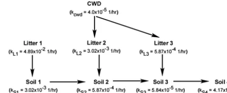
Recently, Koven et al. (2013) used a modified form of the “accelerated decomposition” (hereafter referred to as the AD approach) by numerically increasing the decomposition rates for the two slowest soil carbon pools (named Soil3 C and Soil4 C) to a level so that their turnover rates are similar to the fast pools during the initialization. Numerical evalu-ation found that the approach significantly reduced the spin-up time (Koven et al., 2013). Figure 1 shows the structure of the soil C pool represented in CLM4-CN. Note that het-erotrophic respiration fractions are not shown. The reason that the AD approach can accelerate the spin-up is because these two slowest pools are essentially decoupled from the rest of the ordinary differential equations, in that all other pools do not need input from them. The approach, however, cannot be applied to the coarse woody debris (CWD) pool even though its turnover rate is on the same order of Soil3 C, because it is an input to the litter pools. Changing the rate of CWD will give a different solution of other pools during each integration step using the same initial condition, which will lead to a state far from equilibrium if the state is used in a restart simulation.
In the AD approach, once the solution is obtained from the accelerated run, the state of Soil3 C and Soil4 C can be ana-lytically solved. From Fig. 1, the flux of Soil3 C and Soil4 C pools can be described by the following equations:
dCSoil3
dt = −kS3CSoil3+kS2CSoil2+kL3CLitr3, (1)
dCSoil4
dt = −kS4CSoil4+kS3CSoil3, (2)
wherekL3,kS2,kS3, andkS4are the turnover rates of the Lit-ter3, Soil2, Soil3, and Soil4 C pools shown in Fig. 1, respec-tively. CLitr3, CSoil2, CSoil3and CSoil4are the amount of C in the Litter3, Soil2, Soil3 and Soil4 C pools, respectively. The first term on the right-hand sides of Eqs. (1) and (2) includes heterotrophic respiration. At the steady state, the left-hand sides of Eqs. (1) and (2) become 0; the amount of Soil3 C and Soil4 C can then be solved:
Figure 1. Soil carbon pool structure of CLM4-CN. The arrows
rep-resent the decomposition pathways, andk is the turnover rate of each pool.
CSoil3=
kS2
kS3
CSoil2+
kL3
kS3
CLitr3, (3)
CSoil4=
kS3
kS4
CSoil3. (4)
Equations (3) and (4) are applicable regardless of whether AD or a native run was used (the native run was defined here as the simulations without changing the decomposition rates of Soil3 and Soil4 C pools). Therefore, multiplying Eqs. (3) and (4) by their corresponding accelerator, the results should be close to the native runs. That is,
CSoil3,N= kS2 kS3,N
CSoil2+ kL3 kS3,N
CLitr3=AS3CSoil3, (5) CSoil4,N= kS3
kS4,N
CSoil3=AS4CSoil4, (6)
2 Methods
2.1 Model description
Community land model CLM4 is the land component of the Community Earth System Model (CESM) (Lawrence et al., 2011). Processes simulated in CLM4 include bio-geophysics (solar and longwave radiation, momentum, heat transfer in soil and snow, hydrology of canopy, soil, and snow, and stomatal physiology and photosynthesis) and biogeochemistry (phenology, autotrophic respiration, het-erotrophic respiration, carbon and nitrogen allocation, and nitrogen source/sink). The vegetation structures (leaf area index, stem area index and height) in CLM4-CN are rep-resented through the predictive state variables of leaf and stem carbon, which are coupled to simulate fluxes of carbon and nitrogen state variables in vegetation, litter, and soil or-ganic matter (Lawrence et al., 2011; Thornton and Zimmer-mann, 2007). The tree, shrub and grass plant functional types (PFTs) are divided into tropical, temperate and boreal cli-mate groupings using the PFT physiology and clicli-mate rules of Nemani and Running (1996) and C3/C4 photosynthetic pathways in the case of grasses (Lawrence and Chase, 2007). For this study, we used CLM4-CN in offline mode, which is not coupled to an atmosphere model.
2.2 Gradient projection method
Ifmcis the number of years (one cycle) of atmospheric forc-ing that will be used repeatedly in the spin-up run, we use a spin-up time of [(n+1)mc] years as a stop point for the accelerated decomposition (AD) run, wheren=300/mc is an integer. For example, if the number of years of forcing is mc=7, the stop time will be at year 301. A stop point of ∼300 years for the modified AD approach was selected based on the model results in Koven et al. (2013), but it is not an absolute requirement. The best approach is to stop when NPP reaches a dynamic steady state.
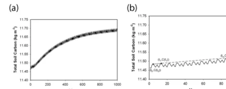
At the end of the accelerated run, a dynamic steady-state water table should be reached in the soil column. Due to the slow turnover rates, the total soil carbon gradually ap-proaches steady state from one cycle to the next (Fig. 2a). We can approximate C at a future timetn(Fig. 2b) using the C gradient between two consecutive cycles expressed in the following equation:
C(tn)=C(t1)+
C(t1)−C(t0)
mc
(tn−t1) , (7)
wheret0 is the beginning of the first cycle,t1 is the begin-ning of the next cycle, andt1−t0=mc;tn−t1=τ mc,τ is an integer close to the turnover years (reciprocal of turnover rate) of the Soil4 C pool to satisfy the stability requirement of forward or explicit time integration that is used in CLM4-CN to solve the time-dependent ordinary differential equa-tions. The explicit method can be numerically unstable (con-vergence of solution is not guaranteed) if the time step is too
Figure 2. Annual average total soil carbon change with respect to
time (a) and the gradient projection over a shorter time interval (b).
big (LeVeque, 2007). For the first-order kinetic type problem, i.e.,u0(t )=ku(t ), the stability requirement is|1+kh| ≤1, in whichkis the rate constant andhis the time step.
We call the method shown in Eq. (7) the gradient projec-tion (GP) method. This method is analogous to that described in Eriksson et al. (2003), which uses a large time step that satisfies the stability requirement for integrating the slowest processes once the contributions from fast processes become negligible. We allowjpto be chosen based on the time pe-riod needed to stabilize the components from fast processes between cycles after perturbation, or set as an integer equal-ingmc×(100/mc+1)years of simulation after restart from the accelerated run before using this approach, and also to performjpyears of simulation followed by each projection until the solution meets the common convergence criteria of 0.5 g m−2for total soil C during two consecutive cycles (Shi et al., 2013; Thornton and Rosenbloom, 2005). During each projection, the balance check for C and N is turned off. The GP method is only applied to the dominant C and N pools, i.e., coarse wood debris, dead stems, dead coarse roots and the Soil4 pool.
3 Results
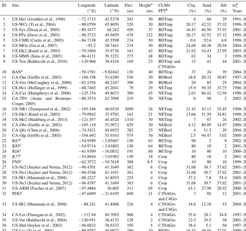
A total of 38 single point tower sites from the FLUXNET (Baldocchi et al., 2001) were selected to assess the gradi-ent projection method. These sites include temperate, bo-real, tropical, and subtropical climatic environments and four ecosystem types (tropical forests, temperate forests, boreal forests, grasslands, and Mediterranean-type ecosystems) (Ta-ble 1).
Table 1. Location, PFT, soil type and number of years of atmospheric forcing for each site.
ID Site Longitude Latitude Elev. Heighta CLM4 Clay Sand Silt mdc
(◦E) (◦N) (m) (m) PFTb (%) (%) (%) Years
1 US-Ha1 (Goulden et al., 1996) −72.1715 42.5378 343 30 BDTmp 6 66 29 1991–2006 2 US-WCr (Yi et al., 2004) −90.0799 45.8059 520 30 BDTmp 20.17 42.52 37.32 1998–2006 3 US-Syv (Desai et al., 2005) −89.3477 46.242 450 37 BDTmp 16.43 46.56 37.01 2001–2006 4 US-PFa (Davis et al., 2003) −90.2723 45.9459 470 122 BDTmp 20.17 42.52 37.32 1995–2005 5 US-UMB (Curtis et al., 2005) −84.7138 45.5598 234 50 BDTmp 0.6 92.6 6.8 1998–2006 6 US-MOz (Gu et al., 2007) −92.2 38.7441 219 30 BDTmp 24.68 46.38 28.94 2004–2007 7 US-Dk2 (Katul et al., 2003) −79.1004 35.9736 163 42 BDTmp 21.62 54.43 23.95 2003–2005 8 US-MMS (Sims et al., 2005) −86.4131 39.3231 275 48 BDTmp 63 34 3 1999–2006 9 US-Ton (Baldocchi et al., 2010) −120.966 38.4316 169 23 BDTmp and
C3NAGrs
15 41 44 2001–2007
10 BANc −50.1591 −9.82442 120 40 BDTrop 37 24 39 2004–2006 11 CA-Oas (Griffis et al., 2003) −106.198 53.6289 530 30 BDBorl 18.8 50.32 30.87 1997–2006 12 CA-Gro (McCaughey et al., 2006) −82.1556 48.2167 300 30 BDBorl 20 65 25 2004–2006 13 US-Ho1 (Hollinger et al., 1999) −68.7403 45.2041 79 29 NETmp 15.9 50.35 33.75 1996–2004 14 CA-Ca1 (Humphreys et al., 2006) −125.334 49.8672 300 45 NETmp 2.63 84.42 12.94 1998–2006 15 CA-TP4 (Arain and
Restrepo-Coupe, 2005)
−80.3574 42.7098 219 30 NETmp 0 98 2 2002–2007
16 US-NR1 (Turnipseed et al., 2002) −105.546 40.0329 3050 26 NETmp 21.43 43.13 35.45 1998–2007 17 US-Dk3 (Katul et al., 2003) −79.0942 35.9782 163 21 NETmp 13.66 51.59 34.81 1998–2005 18 US-Me2 (Hudiburg et al., 2013) −121.557 44.4524 1310 30 NETmp 7 67 26 2002–2007 19 CA-Obs (Griffis et al., 2003) −105.118 53.9872 629 30 NEBorl 4.12 80.89 14.97 2000–2006 20 CA-Qfo (Chen et al., 2006) −74.3421 49.6925 382 25 NEBorl 4 51.5 29 2004–2006 21 CA-Ojp (Griffis et al., 2003) −104.692 53.9163 579 30 NEBorl 2.5 94.47 3.02 2000–2006 22 K67c −54.9589 −2.85667 130 63 BETrop 90 2 8 2002–2004 23 K83c −54.9714 −3.01803 130 64 BETrop 80 18 2 2001–2003 24 RJAc −61.9309 −10.0832 191 60 BETrop 10 80 10 2000–2002 25 K77c −54.8944 −3.01983 130 18 Crop 80 18 2 2001–2005 26 FNSc −62.3572 −10.7618 306 8.5 Crop 10 80 10 1999–2001 27 US-Ne2 (Suyker and Verma, 2012) −96.4701 41.1649 362 6 Crop 31.68 30.7 37.62 2001–2006 28 US-Ne1 (Suyker and Verma, 2012) −96.4766 41.1651 361 6 Crop 31.68 30.7 37.62 2001–2006 29 US-IB1 (Matamala et al., 2008) −88.2227 41.8593 225 4 Crop 37.2 7.8 55.4 2005–2007 30 US-Ne3 (Suyker and Verma, 2012) −96.4397 41.1649 363 6 Crop 31.68 30.7 37.62 2001–2006 31 US-ARM (Fischer et al., 2007) −97.4884 36.605 311 65 Crop 43.1 27.98 28.92 2000–2007 32 PDGc −47.6499 −21.6195 690 21 C3NAGrs
and C4Grs
3 85 12 2001–2003
33 US-IB2 (Matamala et al., 2008) −88.241 41.8406 226 4 C3NAGrs and C4Grs
34.8 12.18 53 2004–2007
34 CA-Let (Flanagan et al., 2002) −112.94 49.7093 960 4 C3NAGrs 35.6 28.1 34.8 1997–2006 35 US-Var (Baldocchi et al., 2004) −120.951 38.4133 129 2 C3NAGrs 12.5 29.5 58 2001–2007 36 US-Shd (Suyker et al., 2003) −96.6833 36.9333 350 5 C3NAGrs 38.4 5.1 56 1997–2000 37 US-Los (Yi et al., 2004) −89.9792 46.0827 480 10 BEShr 16.43 46.56 37.01 2000–2006 38 US-SO2 (Lipson et al., 2005) −116.623 33.3739 1406 5 BEShr 21.31 43.94 34.75 1998–2006
aApproximate height of the wind/temperature and flux measurements above the surface.bAbbreviated PFTs are BDBorl – broadleaf deciduous boreal tree; BDTmp – broadleaf deciduous
temperate tree; BDTrop – broadleaf deciduous tropical tree; BEShr – broadleaf evergreen shrub; BETrop – broadleaf evergreen tropical tree; crop – C3 crop; C3NAGrs – C3 non-arctic grass; C4Grs – C4 grass; NEBorl – needleleaf evergreen boreal tree; and NETmp – needleleaf evergreen temperate tree.cThe site information and meteorological forcing are from the LBA-MIP
data set.dmcis the number of years of atmospheric forcing.
available forcing (Table 1) is applied repeatedly during the simulation for each site.
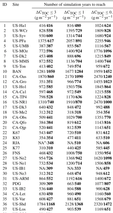
Table 2 shows the comparison of total simulation years till a certain convergence criterion is met. Three convergence threshold values in 1CTOC (3.0, 1.0, and 0.5 g m−2yr−1) were compared. The quality of total soil C is better when the threshold value is smaller (Thornton and Rosenbloom, 2005). Compared to the modified AD approach, the reduc-tion in computareduc-tion cost is shown in Fig. 3. Figure 3 shows that when a high-quality solution (1CTOC≤0.5 g m−2yr−1)
atmo-Table 2. Comparison between the gradient projection method (in
bold) and the accelerated spin-up method.
ID Site Number of simulation years to reach
1CTOC≤3 1CTOC≤1 1CTOC≤0.5
(g m−2yr−1) (g m−2yr−1) (g m−2yr−1)
1 US-Ha1 416/416 816/480 1024/624 2 US-WCr 828/558 1395/729 1809/828 3 US-Syv 930/600 1314/744 1680/924 4 US-PFa 1375/617 2057/891 2255/946 5 US-UMB 387/387 855/567 1116/567 6 US-MOz 772/596 1400/924 1776/1096 7 US-Dk2 453/408 888/696 1215/849 8 US-MMS 872/552 1136/704 1400/744 9 US-Ton 413/402 749/574 959/672 10 BAN 1281/1050 1677/1284 1959/1452 11 CA-Oas 1870/860 2170/1090 2470/1240 12 CA-Gro 351/351 966/774 1455/1023 13 US-Ho1 972/585 1503/756 1845/864 14 CA-Ca1 597/468 972/549 1215/558 15 CA-TP4 798/528 1170/636 1224/828 16 US-NR1 1310/740 1910/870 2470/1000 17 US-Dk3 640/432 848/472 992/488 18 US-Me2 312/312 318/318 354/354 19 CA-Obs 509/441 1029/700 1351/770 20 CA-Qfo 384/384 819/612 1143/816 21 CA-Ojp 520/441 812/539 1143/651 22 K67 543/447 720/510 831/612 23 K83 354/354 477/411 633/510 24 RJA NA∗/348 NA/510 NA/606 25 K77 310/310 440/425 585/445 26 FNS 468/432 1008/750 1350/954 27 US-Ne2 954/726 1368/942 1620/1098 28 US-Ne1 732/534 1200/714 1506/858 29 US-IB1 NA/309 NA/333 NA/459 30 US-Ne3 312/312 648/474 948/612 31 US-ARM 864/552 1192/616 1400/672 32 PDG 309/309 663/540 1077/807 33 US-IB2 536/440 804/588 900/628 34 CA-Let 630/450 960/490 1160/560 35 US-Var 608/427 881/651 1568/679 36 US-Shd 1784/1168 2128/1368 2320/1472 37 US-Los 490/427 903/539 1169/651 38 US-SO2 NA/NA
∗NA – not evaluated
spheric forcing (9 years) (Fig. 4). The oscillation noted in the simulations at RJA and US-IB1 differs from the variabil-ity within the forcing cycle, which happens when soil C has a fast turnover rate such that soil C dynamics are primarily controlled by variability of the forcing (Luo et al., 2014). Due to the aforementioned reasons, the GP method failed at those three sites.
We first checked whether the oscillation and longer peri-odicity were caused by fire disturbance. However, this can only explain the oscillation at site US-SO2. The annual fire disturbance at site US-SO2 is longer than half a year, while it is less than a month at the other two sites. In the original CLM4, soil water is calculated first for the top ten soil
lay-Figure 3. Stacked bar chart of percent reduction in computation cost
for three convergence threshold values.
ers (3.8 m below the ground surface) and one aquifer layer using a water-content-based formulation for water mass con-servation and a groundwater table as the bottom boundary condition (Oleson et al., 2010); the Niu et al. (2005, 2007) parameterizations are then used to simulate groundwater– soil water interaction and update the water table depth. If the water table is below 3.8 m, groundwater does not contribute to the soil moisture in the overlaying soil layers. We found that, after 100 years, the water table calculation scheme in CLM4 has resulted in a significantly different evolution of water table depth from one cycle to the next when repeatedly forcing the model with atmospheric data at sites RJA and US-IB1. The issue has also been found previously and an ef-fort has been made to eliminate the oscillations (Oleson et al., 2010), but such oscillations can still occur under specific conditions such as at RJA and US-IB1. When we turned off the groundwater component, i.e., applying a zero flux bound-ary condition at the bottom of the soil column, we did not see oscillations in SOC at RJA and US-IB1. In the Niu et al. (2007) groundwater model, after solving the mass conser-vation equations (Richards’ equation) in the top ten layers, water is then moved around to account for recharge and sub-surface runoff and in the meantime to satisfy two conditions for water content in each layer; i.e., the water content has to be greater than the minimum content and smaller than the ef-fective porosity of the layer. By moving water mass around after the Richards’ equation is solved, the Richards’ equa-tion at each node is no longer satisfied if its moisture devi-ates from its previous solution. We have confirmed the lo-cal mass conservation error of water in the original model of CLM4. The error is large when recharge or subsurface runoff is high. The water content formulation itself has been previ-ously shown to cause solution instability for soils near sat-uration (Hills et al., 1989). Instead of solving the soil water and groundwater separately, we use a flow model for vari-ably saturated porous media, STOMP (Subsurface Transport Over Multiple Phases) (White and Oostrom, 2000), to see if it can resolve the oscillation in the total soil C.
Figure 4. Annual average total soil C with respect to time at sites
RJA, US-IB1 and US-SO2.
of water mass crossing the control volume surface. The non-linear equations describing mass conservation are discretized spatially on structured orthogonal grids using the integral finite difference approach of Patankar (1980), which is lo-cally and globally mass conserving. The equations are dis-cretized temporally using first-order backward Euler differ-encing or implicit time stepping that is suitable for the solu-tion of the equasolu-tions that are numerically unstable (LeVeque, 2007). Newton–Raphson iteration is used to resolve the non-linearities from the constitutive equations that relate the pri-mary and secondary variables.
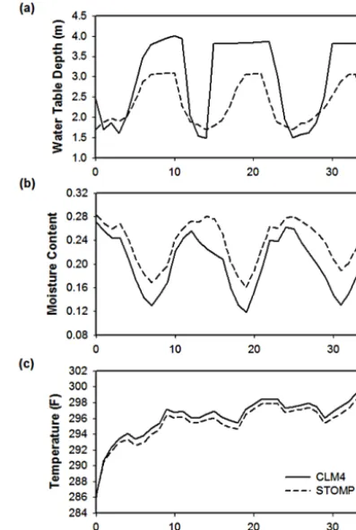
Detailed information regarding STOMP, such as the user’s guide, theory guide and code availability, can be found at http://stomp.pnnl.gov. For each soil column, the number of vertical grids used for STOMP is 15 and it is the same as that in CLM4. In CLM4, the top ten grids (3.8 m below the ground) are used in the soil water scheme. The same initial saturation condition as that in CLM4 is prescribed. For the grid at the top, the Neumann boundary condition is used. For the bottom (42 m below the ground), a zero flux boundary condition is used. Because the aquifer is unconfined, we use the bottom node pressure to calculate water table depth. Fig-ures 5 and 6 show the model comparison at the beginning of the first 3 years between the simulations using the origi-nal soil hydrology scheme in CLM4 and the simulation after
Figure 5. Comparison of water table depth (a), average soil
mois-ture content (b), and average soil temperamois-ture (c) using the original soil hydrology model and STOMP in CLM4 at site RJA.
replacing the soil water and groundwater–soil water interac-tion scheme with STOMP at sites RJA and US-IB1. Using STOMP, mass conservation is improved, and the moisture content calculated is more accurate, resulting in wetter and cooler soil (Figs. 5b, c and 6b, c).
Figure 6. Comparison of water table depth (a), average soil
mois-ture content (b), and average soil temperamois-ture (c) using the original soil hydrology model and STOMP in CLM4 at site US-IB1.
4 Conclusions
We described a gradient projection method to further speed up the spin-up process based on the slow nature of soil or-ganic C decomposition. Comparison between our approach and the modified accelerator approach showed that 20–69 % of simulation years can be reduced with our approach. While the approach was specifically evaluated using CLM4-CN, it can also be readily applied to other CN models in Earth sys-tem models. No matter what modification is made to improve the spin-up efficiency, a final spin-up is always needed to reach a converged solution due to disequilibrium caused by the modification. Our approach is especially useful when a new model formulation is proposed and a high-quality solu-tion (small convergence threshold) is needed for a fair com-parison.
In addition, we also found that the original numerical hy-drology scheme, especially the water table calculation in CLM4, creates numerical oscillations in simulated water ta-bles, leading to a challenge in achieving the common con-vergence criteria for soil C. To resolve the issue, we replaced the hydrological model using a flow model for variably satu-rated porous media. The new flow model caused an increase of about 10 % in computation time, but gives more accurate
Figure 7. Comparison of water table depth simulated by the original
soil hydrology scheme in CLM4 (solid line) and STOMP (dashed line) at site RJA (a) and site US-IB1 (b) in the last 42 years of the simulation; (c) and (d) are annual average total soil carbon at sites RJA and US-IB1 using STOMP in CLM4 and the GP method.
results that corrected the oscillation behavior of the original hydrological model. Comparing the total C predicted by the old and new flow models, we also see more C being predicted using the new flow model. Whether the prediction of more C is realistic depends on other factors besides the hydrology, so we have not attempted to evaluate the simulated C using observations. Nevertheless, a correct implementation of nu-merical schemes is always desirable for reducing uncertainty in model prediction.
Code availability
The source code of CLM4.0 and STOMP can be re-quested through http://www.cesm.ucar.edu/models/cesm1.0/ and http://stomp.pnnl.gov/licensing.stm, respectively. The method implemented in this study can be obtained upon re-quest. Contact: [email protected].
Acknowledgements. This research has been accomplished through
funding support from Pacific Northwest National Laboratory’s Laboratory Directed Research and Development Program. We thank the North American Carbon Program Site-Level Interim Synthesis team, the Large Scale Biosphere-Atmosphere Experi-ment in Amazônia Model Intercomparison Project team, and the site investigators for collecting, organizing, and distributing the data required for this analysis. We thank the anonymous referee and Yiqi Luo for comments that improved the manuscript. A portion of this research was performed using PNNL Institutional Computing at Pacific Northwest National Laboratory. PNNL is operated by Battelle for the US Department of Energy under contract DE-AC05-76RL01830.
References
Arain, A. A. and Restrepo-Coupe, N.: Net ecosystem production in a temperate pine plantation in southeastern Canada, Agr. Forest Meteorol., 128, 223–241, doi:10.1016/j.agrformet.2004.10.003, 2005.
Baldocchi, D., Falge, E., Gu, L. H., Olson, R., Hollinger, D., Running, S., Anthoni, P., Bernhofer, C., Davis, K., Evans, R., Fuentes, J., Goldstein, A., Katul, G., Law, B., Lee, X. H., Malhi, Y., Meyers, W., Oechel, W., Paw U, K. T., Pilegaards, K., Schmid, H. P., Valentini, R., Verma, S., Vesala, T., Wilson, K., and Wofsy, S.: FLUXNET: A new tool to study the temporal and spatial variability of ecosystem-scale carbon dioxide, water va-por, and energy flux densities, B. Am. Meteorol. Soc., 82, 2415– 2434, doi:10.1175/1520-0477(2001)082<2415:Fantts>2.3.Co;2, 2001.
Baldocchi, D. D., Xu, L. K., and Kiang, N.: How plant functional-type, weather, seasonal drought, and soil physical proper-ties alter water and energy fluxes of an oak-grass savanna and an annual grassland, Agr. Forest Meteorol., 123, 13–39, doi:10.1016/j.agrformet.2003.11.006, 2004.
Baldocchi, D. D., Ma, S. Y., Rambal, S., Misson, L., Ourcival, J. M., Limousin, J. M., Pereira, J., and Papale, D.: On the differential advantages of evergreenness and deciduousness in mediterranean oak woodlands: a flux perspective, Ecol. Appl., 20, 1583–1597, doi:10.1890/08-2047.1, 2010.
Birken, P., Gleim, T., Kuhl, D., and Meister, A.: Fast Solvers for Un-steady Thermal Fluid Structure Interaction, arXiv:1407.0893v1, 2014.
Chen, J. M., Govind, A., Sonnentag, O., Zhang, Y. Q., Barr, A., and Amiro, B.: Leaf area index measurements at Fluxnet-Canada forest sites, Agr. Forest Meteorol., 140, 257–268, doi:10.1016/j.agrformet.2006.08.005, 2006.
Curtis, P. S., Vogel, C. S., Gough, C. M., Schmid, H. P., Su, H. B., and Bovard, B. D.: Respiratory carbon losses and the carbon-use efficiency of a northern hardwood forest, 1999–2003, New Phytol., 167, 437–455, doi:10.1111/j.1469-8137.2005.01438.x, 2005.
Davis, K. J., Bakwin, P. S., Yi, C. X., Berger, B. W., Zhao, C. L., Teclaw, R. M., and Isebrands, J. G.: The annual cycles of CO2 and H2O exchange over a northern mixed forest as
ob-served from a very tall tower, Glob. Change Biol., 9, 1278–1293, doi:10.1046/j.1365-2486.2003.00672.x, 2003.
Desai, A. R., Bolstad, P. V., Cook, B. D., Davis, K. J., and Carey, E. V.: Comparing net ecosystem exchange of car-bon dioxide between an old-growth and mature forest in the upper Midwest, USA, Agr. Forest Meteorol., 128, 33–55, doi:10.1016/j.agrformet.2004.09.005, 2005.
Eriksson, K., Johnson, C., and Logg, A.: Explicit time-stepping for stiff ODES, SIAM J. Sci. Comput., 25, 1142–1157, doi:10.1137/S1064827502409626, 2003.
Fang, Y., Huang, M., Liu, C., Li, H., and Leung, L. R.: A generic biogeochemical module for Earth system models: Next Generation BioGeoChemical Module (NGBGC), version 1.0, Geosci. Model Dev., 6, 1977–1988, doi:10.5194/gmd-6-1977-2013, 2013.
Fang, Y., Liu, C., Huang, M., Li, H., and Leung, R.: Steady state estimation of soil organic carbon using satellite-derived canopy leaf area index, Journal of Advances in Modeling Earth Systems, 6, 1049–1064, doi:10.1002/2014MS000331, 2014.
Fischer, M. L., Billesbach, D. P., Berry, J. A., Riley, W. J., and Torn, M. S.: Spatiotemporal variations in growing season exchanges of CO2, H2O, and sensible heat in agricultural fields of the South-ern Great Plains, Earth Interact., 11, 1–21, doi:10.1175/EI231.1, 2007.
Flanagan, L. B., Wever, L. A., and Carlson, P. J.: Seasonal and inter-annual variation in carbon dioxide exchange and carbon balance in a northern temperate grassland, Glob. Change Biol., 8, 599– 615, doi:10.1046/j.1365-2486.2002.00491.x, 2002.
Gear, C. W. and Kevrekidis, I. G.: Projective methods for stiff differential equations: Problems with gaps in their eigen-value spectrum, SIAM J. Sci. Comput., 24, 1091–1106, doi:10.1137/S1064827501388157, 2003.
Goulden, M. L., Munger, J. W., Fan, S. M., Daube, B. C., and Wofsy, S. C.: Measurements of carbon sequestration by long-term eddy covariance: Methods and a critical evaluation of ac-curacy, Glob. Change Biol., 2, 169–182, doi:10.1111/j.1365-2486.1996.tb00070.x, 1996.
Griffis, T. J., Black, T. A., Morgenstern, K., Barr, A. G., Nesic, Z., Drewitt, G. B., Gaumont-Guay, D., and McCaughey, J. H.: Ecophysiological controls on the carbon balances of three southern boreal forests, Agr. Forest Meteorol., 117, 53–71, doi:10.1016/S0168-1923(03)00023-6, 2003.
Gu, L. H., Meyers, T., Pallardy, S. G., Hanson, P. J., Yang, B., Heuer, M., Hosman, K. P., Liu, Q., Riggs, J. S., Sluss, D., and Wullschleger, S. D.: Influences of biomass heat and bio-chemical energy storages on the land surface fluxes and ra-diative temperature, J. Geophys. Res.-Atmos., 112, D02107, doi:10.1029/2007jd008509, 2007.
Hills, R. G., Porro, I., Hudson, D. B., and Wierenga, P. J.: Modeling One-Dimensional Infiltration into Very Dry Soils .1. Model De-velopment and Evaluation, Water Resour. Res., 25, 1259–1269, doi:10.1029/Wr025i006p01259, 1989.
Hollinger, D. Y., Goltz, S. M., Davidson, E. A., Lee, J. T., Tu, K., and Valentine, H. T.: Seasonal patterns and environmen-tal control of carbon dioxide and water vapour exchange in an ecotonal boreal forest, Glob. Change Biol., 5, 891–902, doi:10.1046/j.1365-2486.1999.00281.x, 1999.
Hudiburg, T. W., Law, B. E., and Thornton, P. E.: Evaluation and improvement of the Community Land Model (CLM4) in Ore-gon forests, Biogeosciences, 10, 453–470, doi:10.5194/bg-10-453-2013, 2013.
Humphreys, E. R., Black, T. A., Morgenstern, K., Cai, T. B., Drewitt, G. B., Nesic, Z., and Trofymow, J. A.: Carbon dioxide fluxes in coastal Douglas-fir stands at different stages of develop-ment after clearcut harvesting, Agr. Forest Meteorol., 140, 6–22, doi:10.1016/j.agrformet.2006.03.018, 2006.
Katul, G., Leuning, R., and Oren, R.: Relationship between plant hydraulic and biochemical properties derived from a steady-state coupled water and carbon transport model, Plant Cell Environ., 26, 339–350, doi:10.1046/j.1365-3040.2003.00965.x, 2003. Koven, C. D., Riley, W. J., Subin, Z. M., Tang, J. Y., Torn, M. S.,
Collins, W. D., Bonan, G. B., Lawrence, D. M., and Swenson, S. C.: The effect of vertically resolved soil biogeochemistry and alternate soil C and N models on C dynamics of CLM4, Biogeo-sciences, 10, 7109–7131, doi:10.5194/bg-10-7109-2013, 2013. Lawrence, D. M., Oleson, K. W., Flanner, M. G., Thornton, P.
G.: Parameterization Improvements and Functional and Struc-tural Advances in Version 4 of the Community Land Model, Journal of Advances in Modeling Earth Systems, 3, M03001, doi:10.1029/2011ms000045, 2011.
Lawrence, P. J. and Chase, T. N.: Representing a new MODIS consistent land surface in the Community Land Model (CLM 3.0), J. Geophys. Res.-Biogeosci., 112, G01023, doi:10.1029/2006jg000168, 2007.
LeVeque, R. J.: Finite Difference Methods for Ordinary and Partial Differential Equations: Steady-State and Time-Dependent Prob-lems Society for Industrial and Applied Mathematics, Philadel-phia, PA, 2007.
Lipson, D. A., Wilson, R. F., and Oechel, W. C.: Effects of ele-vated atmospheric CO2on soil microbial biomass, activity, and
diversity in a chaparral ecosystem, Appl. Environ. Microb., 71, 8573–8580, doi:10.1128/Aem.71.12.8573-8580.2005, 2005. Luo, Y., Keenan, T. F., and Smith, M.: Predictability of the
terrestrial carbon cycle, Glob. Change Biol., online first, doi:10.1111/gcb.12766, 2014.
Matamala, R., Jastrow, J. D., Miller, R. M., and Garten, C. T.: Tem-poral changes in C and N stocks of restored prairie: Implica-tions for C sequestration strategies, Ecol. Appl., 18, 1470–1488, doi:10.1890/07-1609.1, 2008.
McCaughey, J. H., Pejam, M. R., Arain, M. A., and Cameron, D. A.: Carbon dioxide and energy fluxes from a boreal mixedwood forest ecosystem in Ontario, Canada, Agr. Forest Meteorol., 140, 79–96, doi:10.1016/j.agrformet.2006.08.010, 2006.
Nemani, R. and Running, S. W.: Implementation of a hierarchical global vegetation classification in ecosystem function models, J. Veg. Sci., 7, 337–346, doi:10.2307/3236277, 1996.
Niu, G. Y., Yang, Z. L., Dickinson, R. E., and Gulden, L. E.: A simple TOPMODEL-based runoff parameterization (SIMTOP) for use in global climate models, J. Geophys. Res.-Atmos., 110, D21106, doi:10.1029/2005jd006111, 2005.
Niu, G. Y., Yang, Z. L., Dickinson, R. E., Gulden, L. E., and Su, H.: Development of a simple groundwater model for use in cli-mate models and evaluation with Gravity Recovery and Cli-mate Experiment data, J. Geophys. Res.-Atmos., 112, D07103, doi:10.1029/2006jd007522, 2007.
Oleson, K. W., Lawrence, D. M., Bonan, G. B., Flanner, M. G., Kluzek, E., Lawrence, P. J., Levis, S., Swenson, S. C., Thornton, P. E., Dai, A., Decker, M., Dickinson, R., Feddema, J., Heald, C. L., Hoffman, F., Lamarque, J.-F., Mahowald, N., Niu, G.-Y., Qian, T., Randerson, J., Running, S., Sakaguchi, K., Slater, A., Stöckli, R., Wang, A., Yang, Z.-L., Zeng, X., and Zeng, X.: Tech-nical Description of version 4.0 of the Community Land Model (CLM). report, 266 pp., Natl. Cent. for Atmos. Res., Boulder, Colo., Rep., 2010.
Patankar, S. V.: Numerical Heat Transfer and Fluid Flow, Hemi-sphere Publishing Corporation, Washington, D.C., 1980. Schwalm, C. R., Williams, C. A., Schaefer, K., Anderson, R., Arain,
M. A., Baker, I., Barr, A., Black, T. A., Chen, G. S., Chen, J. M., Ciais, P., Davis, K. J., Desai, A., Dietze, M., Dragoni, D., Fischer, M. L., Flanagan, L. B., Grant, R., Gu, L. H., Hollinger, D., Izaur-ralde, R. C., Kucharik, C., Lafleur, P., Law, B. E., Li, L. H., Li, Z. P., Liu, S. G., Lokupitiya, E., Luo, Y. Q., Ma, S. Y., Margolis, H., Matamala, R., McCaughey, H., Monson, R. K., Oechel, W. C., Peng, C. H., Poulter, B., Price, D. T., Riciutto, D. M., Riley, W., Sahoo, A. K., Sprintsin, M., Sun, J. F., Tian, H. Q., Tonitto, C.,
Verbeeck, H., and Verma, S. B.: A model-data intercomparison of CO2exchange across North America: Results from the North
American Carbon Program site synthesis, J. Geophys. Res.-Biogeosci., 115, G00H05, doi:10.1029/2009jg001229, 2010. Shi, M. J., Yang, Z. L., Lawrence, D. M., Dickinson, R. E., and
Subin, Z. M.: Spin-up processes in the Community Land Model version 4 with explicit carbon and nitrogen components, Ecol. Model., 263, 308–325, doi:10.1016/j.ecolmodel.2013.04.008, 2013.
Sims, D. A., Rahman, A. F., Cordova, V. D., Baldocchi, D. D., Flanagan, L. B., Goldstein, A. H., Hollinger, D. Y., Misson, L., Monson, R. K., Schmid, H. P., Wofsy, S. C., and Xu, L. K.: Midday values of gross CO2 flux and light use
effi-ciency during satellite overpasses can be used to directly es-timate eight-day mean flux, Agr. Forest Meteorol., 131, 1–12, doi:10.1016/j.agrformet.2005.04.006, 2005.
Suyker, A. E. and Verma, S. B.: Gross primary production and ecosystem respiration of irrigated and rainfed maize-soybean cropping systems over 8 years, Agr. Forest Meteorol., 165, 12– 24, doi:10.1016/j.agrformet.2012.05.021, 2012.
Suyker, A. E., Verma, S. B., and Burba, G. G.: Interan-nual variability in net CO2 exchange of a native tallgrass
prairie, Glob. Change Biol., 9, 255–265, doi:10.1046/j.1365-2486.2003.00567.x, 2003.
Thornton, P. E. and Rosenbloom, N. A.: Ecosystem model spin-up: Estimating steady state conditions in a coupled terrestrial carbon and nitrogen cycle model, Ecol. Model., 189, 25–48, doi:10.1016/j.ecolmodel.2005.04.008, 2005.
Thornton, P. E. and Zimmermann, N. E.: An improved canopy inte-gration scheme for a land surface model with prognostic canopy structure, J. Climate, 20, 3902–3923, doi:10.1175/Jcli4222.1, 2007.
Turnipseed, A. A., Blanken, P. D., Anderson, D. E., and Monson, R. K.: Energy budget above a high-elevation subalpine forest in complex topography, Agr. Forest Meteorol., 110, 177–201, doi:10.1016/S0168-1923(01)00290-8, 2002.
White, M. D. and Oostrom, M.: STOMP Subsurface Transport Over Multiple Phases, Version 2.0, Theory Guide, PNNL-12030, UC-2010, Pacific Northwest National Laboratory, Richland, WA, 2000.
Xia, J. Y., Luo, Y. Q., Wang, Y.-P., Weng, E. S., and Hararuk, O.: A semi-analytical solution to accelerate spin-up of a coupled car-bon and nitrogen land model to steady state, Geosci. Model Dev., 5, 1259–1271, doi:10.5194/gmd-5-1259-2012, 2012.
Yi, C., Davis, K. J., Bakwin, P. S., Denning, A. S., Zhang, N., De-sai, A., Lin, J. C., and Gerbig, C.: Observed covariance between ecosystem carbon exchange and atmospheric boundary layer dy-namics at a site in northern Wisconsin, J. Geophys. Res.-Atmos., 109, D08302, doi:10.1029/2003jd004164, 2004.