Computational Limits of A Distributed Algorithm for Smoothing Spline

Computational Limits of A Distributed Algorithm for

Smoothing Spline

Zuofeng Shang [email protected]

Department of Mathematical Sciences

Indiana University-Purdue University at Indianapolis Indianapolis, IN 46202, USA

Guang Cheng [email protected]

Department of Statistics Purdue University

West Lafayette, IN 47907, USA

Editor:Michael Mahoney

Abstract

In this paper, we explore statistical versus computational trade-off to address a basic ques-tion in the applicaques-tion of a distributed algorithm: what is the minimal computaques-tional cost in obtaining statistical optimality? In smoothing spline setup, we observe a phase transition phenomenon for the number of deployed machines that ends up being a simple proxy for computing cost. Specifically, asharpupper bound for the number of machines is established: when the number is below this bound, statistical optimality (in terms of non-parametric estimation or testing) is achievable; otherwise, statistical optimality becomes impossible. These sharp bounds partly capture intrinsic computational limits of the dis-tributed algorithm considered in this paper, and turn out to be fully determined by the smoothness of the regression function. We name the asymptotic analysis on such split-and-aggregation estimation/inference as “splitotic” theory. As a side remark, we argue that sample splitting may be viewed as an alternative form of regularization, playing a similar role as smoothing parameter.

Keywords: divide-and-conquer, computational limits, smoothing spline, splitotic theory

1. Introduction

In the parallel computing environment, divide-and-conquer (D&C) method distributes data to multiple machines, and then aggregates local estimates computed from each machine to produce a global one. Such a distributed algorithm often requires agrowing number of machines in order to process an increasingly large dataset. A practically relevant question is “how many processors do we really need in this parallel computing?” or “shall we allocate all our computational resources in the data analysis?” Such questions are related to the minimal computational cost of this distributed method (which will be defined more precisely later). The major goal of this paper is to provide some “theoretical” insights, namely, a splitotic theory, for the above questions from a statistical perspective. Specifically, we consider a classical nonparametric regression setup:

yl =f(l/N) +l, l= 0,1, . . . , N−1, (1)

c

wherel’s areiid random errors withE{l}= 0 andV ar(l) = 1, in the following distributed algorithm:

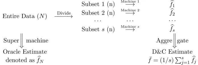
Entire Data (N) −−−−→Divide

Subset 1 (n) Machine 1−→

Subset 2 (n) Machine 2−→

· · · ·

Subset s(n) Machine−→ s

b f1 b f2

· · ·

b fs

Super w w w 

machine Aggre

w w w 

gate

Oracle Estimate D&C Estimate denoted asfb_N f¯= (1/s)

Ps j=1fb_j

We assume that the total sample size isN, the number of machines issand the size of each sub-sample isn. Hence,N =s×n. Each machine produces an individual smoothing spline estimate fb_j to be defined in (3) (Wahba (1990)).

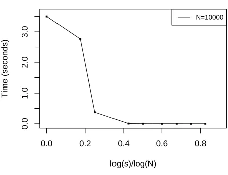
A known property of the above D&C strategy is that it can preserve statistical efficiency for a wide-ranging choice of s (as demonstrated in Figure 1), say logs/logN ∈ [0,0.4], while largely reducing computational burden as logs/logN increases (as demonstrated in Figure 2). An important observation from Figure 1 is that there is an obvious blowup for mean squared errors of ¯f when the above ratio is beyond some threshold, e.g, 0.8 for

N = 10000. Hence, we are interested in knowing whether there exists a critical value of logs/logN in theory, beyond which statistical optimality no longer exists. For example, mean squared errors will never achieve minimax optimal lower bound (at rate level) no matter how smoothing parameters are tuned. Such a sharpness result partly captures the computational limit of the particular D&C algorithm considered in this paper, also complementing the upper bound results in Shang and Cheng (2015); Zhang et al. (2015); Zhao et al. (2016).

Our first contribution is to establish a sharp upper bound of s under which ¯f achieves the minimax optimal rateNm/(2m+1)_{, wheremrepresents the smoothness off}

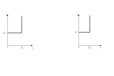
0. By “sharp” upper bound, we mean the largest possible upper bound forsto gain statistical optimality. This result is established by directly computing (non-asymptotic) upper and lower bounds of mean squared error of ¯f. These two bounds holduniformlyassdiverges, and thus imply that the rate of mean squared error transits oncesreaches the rate N2m/(2m+1), which we call as phase transition in divide-and-conquer estimation. In fact, the choice of smoothing parameter, denoted as λ, also plays a very subtle role in the above phase transition. For example,λis not necessarily chosen at an optimal level whensattains the above bound as illustrated in Figure 3.

Our second contribution is a sharp upper bound of s under which a simple Wald-type testing method based on ¯f is minimax optimal in the sense of Ingster (1993). It is not surprising that our testing method is consistent no mattersis fixed or diverges at any rate. Rather, this sharp bound is entirely determined by analyzing its (non-asymptotic) power. Specifically, we find that our testing method is minimax optimal if and only if s does not grow faster thanN(4m−1)/(4m+1). Again, we observe a subtle interplay between sand λas depicted in Figure 3.

Figure 1: Mean-square errors (MSE) off¯based on 500 independent replications under different choices of

Nands. The values of MSE stay at low levels for various choice ofswithlogs/logN∈[0,0.7]. True regression function isf0(z) = 0.6b30,17(z) + 0.4b3,11(z)withba1,a2 the density function for Beta(a1, a2).

0.0 0.2 0.4 0.6 0.8

0.0

1.0

2.0

3.0

log(s)/log(N)

Time (seconds)

N=10000

Figure 2: Computing time off¯based on a single replication under different choices of s whenN= 10,000. The larger thes, the smaller the computing time.

0 b

a

2m 2m+1

2m 2m+1

0 b

a

4m 4m+1

4m−1 4m+1

Figure 3: Two lines indicate the choices ofsNa andλN−b, leading to minimax optimal estimation rate (left) and minimax optimal testing rate (right). Whereas(a, b)’s outside these two lines lead to suboptimal rates. Results are based on smoothing spline regression with regularitym≥1.

we propose to selectλ via a distributed version of generalized cross validation (GCV); see Xu et al. (2017).

In the end, we want to mention that our theoretical results are developed in one-dimensional models under fixed design. This setting allows us to develop proofs based on exact analysis of various Fourier series, coupled with properties of circulant Bernoulli polynomial kernel matrix. The major goal of this work is to provide some theoretical in-sights in a relatively simple setup, which are useful in extending our results to more general setup such as random or multi-dimensional design. Efforts toward this direction have been made by Liu et al. (2017) who derived upper bounds of sfor optimal estimation or testing in various nonparametric models when design is random and multi-dimensional.

2. Smoothing Spline Model

Suppose that we observe samples from model (1). The regression function f is smooth in the sense that it belongs to anm-order (m≥1) periodic Sobolev space:

Sm(I) =

(_∞ X

ν=1

fνϕν(·) : ∞ X

ν=1

f_ν2γν <∞ )

,

whereI:= [0,1] and fork= 1,2, . . .,

ϕ2k−1(t) =

√

2 cos(2πkt), ϕ2k(t) =

√

γ2k−1=γ2k= (2πk)2m.

The entire dataset is distributed to each machine in a uniform manner as follows. For

j= 1, . . . , s, thejth machine is assigned with samples (Yi,j, ti,j), where

Yi,j =yis−s+j−1 and ti,j =

is−s+j−1

N

fori= 1, . . . , n. Obviously,t1,j, . . . , tn,j are evenly spaced points (with a gap 1/n) acrossI.

At the jth machine, we have the following sub-model:

Yi,j =f(ti,j) +i,j, i= 1, . . . , n, (2) wherei,j =is−s+j−1, and obtain the jth sub-estimate as

b

fj = arg min f∈Sm₍

I)`j,n,λ(f).

Here,`j,n,λ represents a penalized square criterion function based on the jth subsample:

`j,n,λ(f) = 1 2n

n X

i=1

(Yi,j−f(ti,j))2+

λ

2J(f, f), (3)

withλ >0 being a smoothing parameter andJ(f, g) =R

If

(m)_(t)g(m)_(t)dt1

3. Minimax Optimal Estimation

In this section, we investigate the impact of the number of machines on the mean squared error of ¯f. Specifically, Theorem 3.1 provides an (non-asymptotic) upper bound for this mean squared error, while Theorem 3.2 provides a (non-asymptotic) lower bound. Notably, both bounds hold uniformly as s diverges. From these bounds, we observe an interesting phase transition phenomenon that ¯f is minimax optimal if s does not grow faster than

N2m/(2m+1) and an optimalλN−2m/(2m+1) is chosen, but the minimax optimality breaks down if sgrows even slightly faster (no matter howλ is chosen). Hence, the upper bound of s is sharp. Moreover, λ does not need to be optimal when this bound is attained. In some sense, a proper sample splitting can compensate a sub-optimal choice of λ.

In this section, we assume that l’s areiid zero-mean random variables with unit vari-ance. Denote mean squared error as

MSEf0(f) :=Ef0{kf−f0k

2 2}, wherekfk2 =

q R

If(t)

2_{dt. For simplicity, we writeE}

f0 asE later. Defineh=λ

1/(2m)_. Theorem 3.1 (Upper Bounds of Variance and Squared Bias) Suppose h > 0, and N is divisible by n. Then there exist absolute positive constants bm, cm ≥ 1 (depending on m

only) such that

E{kf¯−E{f¯}k2 2} ≤bm

N−1+ (N h)−1 Z πnh

0

1

(1 +x2m₎2dx

, (4)

kE{f¯} −f0k2≤cm p

J(f0)(λ+n−2m+N−1) (5)

for any fixed 1≤s≤N.

From (17) and (18) in Appendix, we can tell that ¯f −E{f¯} is irrelevant to f0. So is the upper bound for the (integrated) variance in (4). However, this is not the case for the (integrated) biaskE{f¯} −f0k2, whose upper bound depends on f0 through its normJ(f0). In particular, the (integrated) bias becomes zero if f0 is in the null space, i.e., J(f0) = 0, according to (5).

Since

MSEf0( ¯f) =E{kf¯−E{f¯}k

2

2}+kE{f¯} −f0k22, (6) Theorem 3.1 says that

MSEf0( ¯f)≤bm

N−1+ (N h)−1 Z πnh

0

1

(1 +x2m₎2dx

+c2_mJ(f0)(λ+n−2m+N−1). (7)

When we choose h N−1/(2m+1) and n−2m =O(λ), it can be seen from (7) that ¯f is minimax optimal, i.e., kf¯−f0k2 =OP(N−m/(2m+1)). Obviously, the above two conditions hold if

λN−2m/(2m+1) and s=O(N2m/(2m+1)). (8) From now on, we define the optimal choice ofλas N−2m/(2m+1), denoted asλ∗; according to Zhang et al. (2015). Alternatively, the minimax optimality can be achieved if s

N2m/(2m+1) and nh = o(1), i.e., λ = o(λ∗). In other words, a sub-optimal choice of λ

can be compensated by a proper sampling splitting strategy. See Figure 3 for the subtle relation between s and λ. It should be mentioned that λ∗ depends on N (rather than n) for achieving optimal estimation rate. In practice, we propose to selectλvia a distributed version of GCV; see Xu et al. (2017).

Remark 3.1 Under random design and uniformly bounded eigenfunctions, Corollary 4 in Zhang et al. (2015) showed that the above rate optimality is achieved under the following upper bound on s(and λ=λ∗)

s=O(N(2m−1)/(2m+1)/logN).

For example, when m= 2, their upper bound is N0.6/logN (versus N0.8 in our case). We improve their upper bound by applying a more direct proof strategy.

To understand whether our upper bound can be further improved, we prove a lower bound result in a “worst case” scenario. Specifically, Theorem 3.2 implies that once s is beyond the above upper bound, the rate optimality will break down for at least one true

f0.

Theorem 3.2 (Lower Bound of Squared Bias) Suppose h > 0, and N is divisible by n. Then for any constantC >0, it holds that

sup f0∈Sm(I)

J(f0)≤C

kE{f¯} −f0k22 ≥C(amn−2m−8N−1),

It follows by (6) that

sup f0∈Sm(I)

J(f0)≤C

MSEf0( ¯f)≥ sup

f0∈Sm(I) J(f0)≤C

kE{f¯} −f0k22≥C(amn−2m−8N−1). (9)

It is easy to check that the above lower bound is strictly slower than the optimal rate

N−2m/(2m+1) ifs grows faster thanN2m/(2m+1) no matter how λis chosen. Therefore, we claim that N2m/(2m+1) _{is a sharp upper bound of s for obtaining an averaged smoothing} spline estimate.

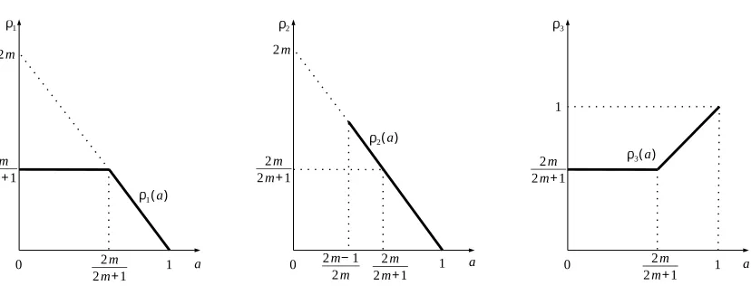
In the end, we provide a graphical interpretation for our sharp bound result. Lets=Na

for 0≤a≤1 andλ=N−b for 0< b <2m. Define ρ1(a), ρ2(a) and ρ3(a) as Upper bound of squared bias:N−ρ1(a) _λ+n−2m_+N−1_,

Lower bound of squared bias:N−ρ2(a) _max{n−2m_−N−1_,0},

Upper bound of variance:N−ρ3(a) _N−1_{+ (N h)}−1 Z πnh

0

1

(1 +x2m₎2dx, based on Theorems 3.1 and 3.2. A direct examination reveals that

ρ1(a) = min{2m(1−a),1, b}

ρ2(a) =

2m(1−a), a >(2m−1)/(2m)

∞, a≤(2m−1)/(2m)

ρ3(a) = max{a,(2m−b)/(2m)}

Figure 4 displaysρ1, ρ2, ρ3forλ=N−2m/(2m+1). It can be seen that whena∈[0,2m/(2m+ 1)], upper bounds of squared bias and variance maintain at the same optimal rateN−2m/(2m+1), while the exact bound of squared bias increases aboveN−2m/(2m+1) when a∈(2m/(2m+ 1),1). This explains why transition occurs at the critical pointa= 2m/(2m+1) (even when the upper bound of variance decreases below N−2m/(2m+1) when a∈(2m/(2m+ 1),1)).

It should be mentioned that when λ6=N−2m/(2m+1), i.e.,b6= 2m/(2m+ 1), suboptimal estimation almost always occurs. More explicitly,b <2m/(2m+1) yieldsρ1(a)<2m/(2m+ 1) for any 0 ≤ a ≤ 1. While b > 2m/(2m + 1) yields ρ2(a) < 2m/(2m+ 1) for any 2m/(2m+ 1) < a≤ 1; yields ρ3(a) < 2m/(2m+ 1) for any 0 ≤ a < 2m/(2m+ 1). The only exception is a = 2m/(2m+ 1) which yields ρ1 = ρ2 = ρ3 = 2m/(2m+ 1) for any

b >2m/(2m+ 1).

Remark 3.2 As a side remark, we notice that each machine is assigned withnN1/(2m+1)

samples when s attains its upper bound in the estimation regime. This is very similar as the local polynomial estimation where approximately N1/(2m+1) _{local points are used for}

obtaining optimal estimation (although we realize that our data is distributed in a global manner).

1

2m

2m+1

1(a)

a

0 2m

1

2m

2m+1

2m

1 2m

2m+1

2(a)

a 0

2

2m 2m+1 2m₋1

2m

1 2m

2m+1

3(a)

a

0 1

3

2m

2m+1

Figure 4: Plots of ρ1(a), ρ2(a), ρ3(a) versus a, indicated by thick solid lines, under λ = N−2m/(2m+1).

ρ1(a), ρ2(a) and ρ3(a) indicate upper bound of squared bias, lower bound of squared bias and upper bound of variance, respectively. ρ2(a) is plotted only for (2m−1)/(2m)< a ≤1; when

0≤a≤(2m−1)/(2m),ρ2(a) =∞, which is omitted.

4. Minimax Optimal Testing

In this section, we consider nonparametric testing:

H0:f = 0 v.s. H1 :f ∈Sm(I)\{0}. (10)

In general, testingf =f0 (for a knownf0) is equivalent to testingf∗≡f−f0= 0. So (10) has no loss of generality. Inspired by the classical Wald test (Shao (2003)), we propose a simple test statistic based on the ¯f as

TN,λ:=kf¯k22.

We find that testing consistency essentially requires no condition on the number of machines no matter it is fixed or diverges at any rate. However, our power analysis, which is non-asymptotically valid, depends on the number of machines in a nontrivial way. Specifically, we discover that our test method is minimax optimal in the sense of Ingster (Ingster (1993)) whensdoes not grow faster thanN(4m−1)/(4m+1) andλis chosen optimally (different from

λ∗, though), but it is no longer optimal oncesis beyond the above threshold (no matter how

λis chosen). This is a similar phase transition phenomenon as we observe in the estimation regime. Again, we notice an optimal choice of λmay not be necessary if the above upper bound ofsis achieved.

assuming Gaussian errors. This extension is possible (technically tedious, though) since likelihood ratio statistic can be approximated by TN,λ through quadratic expansion; see Shang and Cheng (2013).

Theorem 4.1 implies the consistency of our proposed test method with the following testing rule:

φN,λ=I(|TN,λ−µN,λ| ≥z1−α/2σN,λ), whereµN,λ:= EH0{TN,λ},σ

2

N,λ:= VarH0{TN,λ}andz1−α/2 is the (1−α/2)×100 percentile

of N(0,1). The conditions required in Theorem 4.1 are so mild that our proposed testing is consistent no matter the number of machines is fixed or diverges at any rate.

Theorem 4.1 (Testing Consistency) Suppose that h → 0, n → ∞ when N → ∞, and

limN→∞nh exists (which could be infinity). Then, we have under H0,

TN,λ−µN,λ

σN,λ d

−→N(0,1), as N → ∞.

Our next theorem analyzes the non-asymptotic power ofTN,λ, in which we pay particular attention to the impact of son the separation rate of testing, defined as

dN,λ= q

λ+n−2m+σN,λ.

LetB={f ∈Sm(I) :J(f)≤C}for a positive constant C.

Theorem 4.2 (Upper Bound) Suppose thath→0,n→ ∞whenN → ∞, andlimN→∞nh

exists (which could be infinity). Then for any ε > 0, there exist Cε, Nε > 0 s.t. for any

N ≥Nε,

inf f∈B kfk2≥CεdN,λ

Pf(φN,λ= 1)≥1−ε. (11)

Under assumptions of Theorem 4.1, it can be shown that (see (55) in Appendix)

σ_N,λ2

_n

N2, if limN→0nh= 0,

1

N2_h, if limN→∞nh >0.

(12)

Given a range ofλleading to limN→∞nh >0, we have by (12) thatdN,λ= p

λ+ (N h1/2₎−1_. An optimal choice of λ (satisfying the above requirement) is λ∗∗ := N−4m/(4m+1) since it leads to the optimal separating rate d∗_N,λ:= N−2m/(4m+1); see Ingster (1993). Meanwhile, the constraint limN→∞nh >0 (together with the choice ofλ∗∗) implies that

s=O(N(4m−1)/(4m+1)). (13)

The above discussions illustrate that we can always chooseλ∗∗to obtain a minimax optimal testing (just as in the single dataset Shang and Cheng (2013)) as long ass does not grow faster than N(4m−1)/(4m+1). In the case that limN→∞nh= 0, the minimax optimality can be maintained if sN(4m−1)/(4m+1), h =o(1) and nh=o(1). Such a selection of sgives us a lot of freedom in choosing λ that needs to satisfyλ =o(λ∗∗). A complete picture in depicting the relation betweensand λis given in Figure 3.

Theorem 4.3 (Lower Bound) Suppose that s N(4m−1)/(4m+1), h → 0, n → ∞ when

N → ∞, and limN→∞nh exists (which could be infinity). Then there exists a positive sequenceβN,λ withlimN→∞βN,λ=∞ s.t.

lim sup N→∞

inf f∈B kfk2≥βN,λd∗N,λ

Pf(φN,λ= 1)≤α. (14)

Recall that1−α is the pre-specified significance level.

Theorem 4.3 says that whensN(4m−1)/(4m+1), the test φN,λ is no longer powerful even when kfk2 d∗_N,λ. In other words, our test method fails to be optimal. Therefore, we claim thatN(4m−1)/(4m+1)is a sharp upper bound ofsto ensure our testing to be minimax optimal.

Remark 4.1 As a side remark, the existence oflimN→∞nhcan be replaced by the following

weaker condition under which the results in Theorems 4.1, 4.2 and 4.3 still hold:

Condition (R):either lim

N→∞nh= 0 or N≥1inf nh >0.

Condition (R) aims to exclude irregularly behaved s such as in the following case where s

vibrates too much along with N:

s=

Nb1_{, N is odd,}

Nb2_{, N is even,} (15)

where h N−c for some c > 0, b1, b2 ∈ [0,1] satisfy b1+c ≥ 1 and b2+c < 1. Clearly,

Condition (R) fails under (15).

5. Discussions

This paper offers “theoretical” suggestions on the allocation of data. In a relatively sim-ple distributed algorithm, i.e., in m-order periodic splines with evenly spaced design, our recommendation proceeds as follows:

• Distribute to

sN2m/(2m+1)

machines for obtaining an optimal estimate;

• Distribute to

sN(4m−1)/(4m+1)

machines for performing an optimal test.

Another theoretically interesting direction is how much adaptive estimation (where m is unknown) can affect the computational limits.

Acknowledgments

We thank PhD student Meimei Liu at Purdue for the simulation study. Zuofeng Shang’s research is sponsored by NSF DMS-1764280. Guang Cheng’s research is sponsored by NSF (CAREER Award DMS-1151692, DMS-1418042), Simmons Fellowship in Mathematics and OCE of Naval Research (ONR N00014-15-1-2331). Guang Cheng gratefully acknowledges Statistical and Applied Mathematical Sciences Institute (SAMSI) for the hospitality and support during his visit in the 2013-Massive Data Program.

6. Appendix

Proofs of our results are included in this section.

6.1 Proofs in Section 3

Proof [Proof of Theorem 3.1] We do a bit preliminary analysis before proving (4) and (5). It follows from Wahba (1990) that (Sm₍

I), J) is a reproducing kernel Hilbert space with

reproducing kernel function

K(x, y) = ∞ X

ν=1

ϕν(x)ϕν(y)

γν

= 2 ∞ X

k=1

cos(2πk(x−y))

(2πk)2m , x, y∈I.

For convenience, define Kx(·) = K(x,·) for any x ∈ I. It follows from the representer

theorem (Wahba (1990)) that the optimization to problem (3) has a solution

b fj =

n X

i=1 b

ci,jKti,j, j = 1,2, . . . , s, (16)

where_bcj = (bc1,j, . . . ,bcn,j)

T _=n−1_(Σ

j+λIn)−1Yj,Yj = (Y1,j, . . . , Yn,j)T,Inisn×nidentity matrix, and Σj = [K(ti,j, ti0_,j)/n]_1≤i,i0_≤n. It is easy to see that Σ₁ = Σ₂ =· · · = Σ_s. For

convenience, denote Σ = Σ1. Similarly, define

K0(x, y) = ∞ X

ν=1

ϕν(x)ϕν(y)

γ2 ν

= 2 ∞ X

k=1

cos(2πk(x−y))

(2πk)4m , x, y∈I.

For 1≤j ≤s, let Ωj = [K0(ti,j, ti0_,j)/n]_1≤i,i0_≤n. It is easy to see that Ω₁ = Ω₂ =· · ·= Ω_s.

For convenience, denote Ω = Ω1, and let Φν,j = (ϕν(t1,j), . . . , ϕν(tn,j)). It is easy to examine that

¯

f =

∞ X

ν=1 Ps

j=1Φν,j(Σ +λIn)−1Yj

N γν

ϕν

= ∞ X

ν=1 Ps

j=1Φν,j(Σ +λIn)−1(f0,j+j)

N γν

and

E{f¯}= ∞ X

ν=1 Ps

j=1Φν,j(Σ +λIn)−1f0,j

N γν

ϕν, (18)

wheref0,j = (f0(t1,j), . . . , f0(tn,j))T andj = (1,j, . . . , n,j)T. We now look at Σ and Ω. For 0≤l≤n−1, let

cl = 2

n

∞ X

k=1

cos(2πkl/n) (2πk)2m ,

dl = 2

n

∞ X

k=1

cos(2πkl/n) (2πk)4m .

Since cl=cn−l and dl =dn−l forl= 1,2, . . . , n−1, Σ and Ω are both symmetric circulant of ordern. Letε= exp(2π√−1/n). Ω and Σ share the same normalized eigenvectors as

xr= 1

√

n(1, ε

r_{, ε}2r_{, . . . , ε}(n−1)r₎T_{, r= 0,1, . . . , n−1.}

LetM = (x0, x1, . . . , xn−1). DenoteM∗ as the conjugate transpose ofM. Clearly,M M∗=

In and Σ,Ω admits the following decomposition

Σ =MΛcM∗, Ω =MΛdM∗, (19)

where Λc = diag(λc,0, λc,1, . . . , λc,n−1) and Λd = diag(λd,0, λd,1, . . . , λd,n−1) with λc,l =

c0+c1εl+. . .+cn−1ε(n−1)l and λd,l =d0+d1εl+. . .+dn−1ε(n−1)l. Direct calculations show that

λc,l= (

2P∞

k=1 (2πkn)1 2m, l= 0,

P∞

k=1[2π(kn−l)]1 2m +

P∞

k=0[2π(kn+l)]1 2m, 1≤l≤n−1.

(20)

λd,l= (

2P∞

k=1(2πkn)1 4m, l= 0,

P∞ k=1

1

[2π(kn−l)]4m +

P∞ k=0

1

[2π(kn+l)]4m, 1≤l≤n−1.

(21)

It is easy to examine that

λc,0 = 2¯cm(2πn)−2m, λd,0 = 2 ¯dm(2πn)−4m, (22)

and for 1≤l≤n−1,

λc,l =

1

[2π(n−l)]2m + 1 (2πl)2m +

∞ X

k=2

1

[2π(kn−l)]2m + ∞ X

k=1

1

[2π(kn+l)]2m,

λd,l =

1

[2π(n−l)]4m + 1 (2πl)4m +

∞ X

k=2

1

[2π(kn−l)]4m + ∞ X

k=1

1

and for ¯cm:=P∞k=1k−2m,cm:= P∞

k=2k−2m, ¯dm:=P∞k=1k−4m,dm:= P∞

k=2k−4m,

c_m(2πn)−2m ≤

∞ X

k=2

1

[2π(kn−l)]2m ≤c¯m(2πn) −2m_,

c_m(2πn)−2m ≤

∞ X

k=1

1

[2π(kn+l)]2m ≤c¯m(2πn) −2m_,

d_m(2πn)−4m ≤

∞ X

k=2

1

[2π(kn−l)]4m ≤d¯m(2πn) −4m

,

d_m(2πn)−4m ≤

∞ X

k=1

1

[2π(kn+l)]4m ≤d¯m(2πn) −4m_.

For simplicity, we denote I = E{kf¯−E{f¯}k2

2} and II = kE{f¯} − f0k22. Hence, MSEf0( ¯f) =I+II.

Using (19) – (23), we get that

I =

∞ X

ν=1 Ps

j=1E{|Φν,j(Σ +λIn)−1j|2}

N2_γ2 ν

= ∞ X

ν=1 Ps

j=1trace((Σ +λIn)−1Φν,jT Φν,j(Σ +λIn)−1)

N2_γ2 ν

= n

N2 s X

j=1

trace (Σ +λIn)−1 ∞ X

ν=1

ΦT_ν,jΦν,j/n

γ2 ν

(Σ +λIn)−1 !

= n

N2 s X

j=1

trace (Σ +λIn)−1Ω(Σ +λIn)−1

= 1

Ntrace M(Λc+λIn)

−1_Λ

d(Λc+λIn)−1M∗

= 1

N

n−1 X

l=0

λd,l (λ+λc,l)2

≤ 2 ¯dm

N(2¯cm+ (2πn)2mλ)2 +(1 + ¯dm)N−1

n−1 X

l=1

(2π(n−l))−4m+ (2πl)−4m (λ+ (2π(n−l))−2m_{+ (2πl)}−2m₎2

≤ 2 ¯dm

N(2¯cm+ (2πn)2mλ)2 +2(1 + ¯dm)N−1

X

1≤l≤n/2

(2πl)−4m+ (2π(n−l))−4m (λ+ (2πl)−2m_{+ (2π(n−l))}−2m₎2

≤ 2 ¯dm

N(2¯cm+ (2πn)2mλ)2

+ 4(1 + ¯dm)N−1 X

1≤l≤n/2

(2πl)−4m (λ+ (2πl)−2m₎2

≤ 2 ¯dm

N(2¯cm+ (2πn)2mλ)2

+2(1 + ¯dm)

πN h

Z πnh 0

1

(1 +x2m₎2dx

≤ bm

1

N +

1

N h Z πnh

0

1

(1 +x2m₎2dx

,

wherebm ≥1 is an absolute constant depending on m only. This proves (4). Proof of (5)

Throughout, let η= exp(2π√−1/N). For 1≤j, l≤s, define

Σj,l = 1

n

∞ X

ν=1

ΦT_ν,jΦν,l

γν

,

σj,l,r = 2

n

∞ X

k=1

cos2πk_nr −j−l_N

It can be shown that Σj,l is a circulant matrix with elementsσj,l,0, σj,l,1, . . . , σj,l,n−1, there-fore, by Brockwell and Davis (1987) we get that

Σj,l=MΛj,lM∗, (24)

where M is the same as in (19), and Λj,l = diag(λj,l,0, λj,l,1, . . . , λj,l,n−1), with λj,l,r, for

r= 1, . . . , n−1, given by the following

λj,l,r = n−1 X

t=0

σj,l,tεrt

= 2

n

n−1 X

t=0 ∞ X

k=1 cos

2πk

t n−

j−l N

(2πk)2m ε rt

= 1

n

∞ X

k=1

η−k(j−l)Pn−1

t=0 ε(k+r)t+ηk(j−l) Pn−1

t=0 ε(r−k)t (2πk)2m

= ∞ X

q=1

η−(qn−r)(j−l)

[2π(qn−r)]2m + ∞ X

q=0

η(qn+r)(j−l)

[2π(qn+r)]2m, (25) and for r= 0, given by

λj,l,0 = n−1 X

t=0

σj,l,t

= 1

n

∞ X

k=1 Pn−1

t=0 εktηk(j−l)+ Pn−1

t=0 ε−ktη−k(j−l) (2πk)2m

= ∞ X

q=1

ηqn(j−l)+η−qn(j−l)

(2πqn)2m . (26)

For p≥0, 1≤v≤n, 0≤r ≤n−1 and 1≤j≤s, define

Ap,v,r,j = 1

s

s X

l=1

λj,l,rx∗rΦT2(pn+v)−1,l, Bp,v,r,j = 1

s

s X

l=1

λj,l,rx∗rΦT2(pn+v),l.

By direct calculation, we have for 1≤v≤n−1,

Φ2(pn+v)−1,lxr = p

n/2η(pn+v)(l−1)I(r+v=n) +η−(pn+v)(l−1)I(v=r),

Φ2(pn+v),lxr = p

−n/2

η(pn+v)(l−1)I(r+v=n)−η−(pn+v)(l−1)I(v=r)

,

(27)

and

Φ2(pn+n)−1,lxr = p

n/2I(r = 0)η(p+1)n(l−1)+η−(p+1)n(l−1),

Φ2(pn+n),lxr = p

−n/2I(r= 0)

η(p+1)n(l−1)−η−(p+1)n(l−1)

LetI(·) be an indicator function. Then we have forp≥0, 1≤j≤sand 1≤v, r≤n−1,

Bp,v,r,j = 1

s

s X

l=1

λj,l,rx∗rΦT2(pn+v),l

= −1

s p

−n/2 s X

l=1 

 ∞ X

q=1

η−(qn−r)(j−l)

[2π(qn−r)]2m + ∞ X

q=0

η(qn+r)(j−l)

[2π(qn+r)]2m 



×η−(pn+v)(l−1)I(r+v=n)−η(pn+v)(l−1)I(r=v)

= −p−n/2 

 X

u≥−p/s

η−(pn+v)(j−1)

[2π(uN+pn+v)]2mI(r+v=n)

− X

u≥(p+1)/s

η(pn+v)(j−1)

[2π(uN−pn−v)]2mI(r=v)

+ X

u≥(p+1)/s

η−(pn+v)(j−1)

[2π(uN−pn−v)]2mI(r+v=n)

− X

u≥−p/s

η(pn+v)(j−1)

[2π(uN+pn+v)]2mI(r=v) 

=a_p,vx∗_rΦT_2(pn+v),j, (29)

where ap,v = P

u≥−p/s[2π(uN+pn+v)]1 2m +

P

u≥(p+1)/s [2π(uN−pn−v)]1 2m, for p ≥ 0, 1 ≤ v ≤

n−1.

For v=n, similar calculations give that

Bp,n,r,j = − p

−n/2I(r= 0) 

 X

u≥−p/s

η−(pn+n)(j−1)

[2π(uN+pn+n)]2m

− X

u≥(p+2)/s

η(pn+n)(j−1)

[2π(uN−pn−n)]2m

+ X

u≥(p+2)/s

η−(pn+n)(j−1)

[2π(uN−pn−n)]2m − X

u≥−p/s

η(pn+n)(j−1)

[2π(uN+pn+n)]2m 



= ap,nx∗rΦT2(pn+n),j, (30)

whereap,n=Pu≥−p/s[2π(uN+pn+n)]1 2m +

P

Similarly, we have p≥0, 1≤j≤sand 1≤v, r≤n−1,

Ap,v,r,j = p

n/2 

 X

u≥−p/s

η−(pn+v)(j−1)

[2π(uN+pn+v)]2mI(r+v=n)

+ X

u≥(p+1)/s

η(pn+v)(j−1)

[2π(uN−pn−v)]2mI(r=v)

+ X

u≥(p+1)/s

η−(pn+v)(j−1)

[2π(uN−pn−v)]2mI(r+v=n)

+ X u≥−p/s

η(pn+v)(j−1)

[2π(uN+pn+v)]2mI(r=v) 

=ap,vx∗rΦT2(pn+v)−1,j, (31)

and for v=n,

Ap,n,r,j = p

n/2I(r= 0) 

 X

u≥−p/s

η−(pn+n)(j−1)

[2π(uN+pn+n)]2m

+ X

u≥(p+2)/s

η(pn+n)(j−1)

[2π(uN−pn−n)]2m + X

u≥(p+2)/s

η−(pn+n)(j−1)

[2π(uN−pn−n)]2m

+ X u≥−p/s

η(pn+n)(j−1)

[2π(uN+pn+n)]2m 

=a_p,nx∗_rΦT_{2(pn+n)−1,j}. (32)

It is easy to check that both (29) and (31) hold forr = 0. Summarizing (29)–(32), we have that forp≥0, 1≤j≤s, 1≤v≤n and 0≤r ≤n−1,

Ap,v,r,j = ap,vx∗rΦT2(pn+v)−1,j,

Bp,v,r,j = ap,vx∗rΦT2(pn+v),j. (33) To show (5), let f¯_j = (E{f¯(t1,j)}, . . . , E{f¯(tn,j)})T, for 1 ≤j ≤ s. It follows by (18) that

¯

f_j =

∞ X

ν=1 Ps

l=1Φν,l(Σ +λIn) −1_f0,l

N γν

ΦT_ν,j

= 1

s

s X

l=1 1

n

∞ X

ν=1 ΦT

ν,jΦν,l

γν !

(Σ +λIn)−1f0,l

= 1

s

s X

l=1

Σj,l(Σ +λIn)−1f0,l

= 1

s

s X

l=1

together with (33), leading to that

M∗f¯_j = 1

s

s X

l=1

Λj,l(Λc+λIn)−1M∗f0,l

= ∞ X

µ=1

f_µ0      1 s Ps

l=1λj,l,0x∗0ΦTµ,l

λ+λc,0

.. .

1

s

Ps

l=1λj,l,n−1x∗n−1ΦTµ,l

λ+λc,n−1

     = ∞ X p=0 n X v=1

f_2(pn+v)−10      1 s Ps

l=1λj,l,0x∗0ΦT2(pn+v)−1,l

λ+λc,0

.. .

1

s

Ps

l=1λj,l,n−1x∗n−1ΦT2(pn+v)−1,l

λ+λc,n−1

     + ∞ X p=0 n X v=1

f_2(pn+v)0      1 s Ps

l=1λj,l,0x∗0ΦT2(pn+v),l

λ+λc,0

.. .

1

s

Ps

l=1λj,l,n−1x∗n−1ΦT2(pn+v),l

λ+λc,n−1

     = ∞ X p=0 n X v=1

f_2(pn+v)−10 

  

Ap,v,0,j

λ+λc,0

.. . Ap,v,n−1,j

λ+λc,n−1     + ∞ X p=0 n X v=1

f_2(pn+v)0 

  

Bp,v,0,j

λ+λc,0

.. . Bp,v,n−1,j

λ+λc,n−1     = ∞ X p=0 n X v=1

f_2(pn+v)−10 

 

ap,v

λ+λc,0x

∗

0ΦT2(pn+v)−1,j ..

. ap,v

λ+λc,n−1x

∗

n−1ΦT2(pn+v)−1,j    + ∞ X p=0 n X v=1

f_2(pn+v)0 

 

ap,v

λ+λc,0x

∗

0ΦT2(pn+v),j ..

. ap,v

λ+λc,n−1x

∗

n−1ΦT2(pn+v),j 

 .

On the other hand,

M∗f0,j = ∞ X

µ=1

f_µ0M∗ΦT_µ,j

= ∞ X p=0 n X v=1

f_2(pn+v)−10 M∗ΦT_{2(pn+v)−1,j}+ ∞ X p=0 n X v=1

f_2(pn+v)0 M∗ΦT_2(pn+v),j

= ∞ X p=0 n X v=1

f_2(pn+v)−10 

 

x∗₀ΦT_{2(pn+v)−1,j} .. .

x∗n−1ΦT2(pn+v)−1,j   + ∞ X p=0 n X v=1

f_2(pn+v)0 

 

x∗₀ΦT_2(pn+v),j .. .

x∗n−1ΦT2(pn+v),j 

Therefore,

M∗(f¯_j−f0,j) = ∞ X p=0 n X v=1

f_2(pn+v)−10 

 

bp,v,0x∗0ΦT2(pn+v)−1,j ..

.

bp,v,n−1x∗n−1ΦT2(pn+v)−1,j    + ∞ X p=0 n X v=1

f_2(pn+v)0 

 

bp,v,0x∗0ΦT2(pn+v),j ..

.

bp,v,n−1x∗n−1ΦT2(pn+v),j 



, (34)

wherebp,v,r = _λ+λap,v_c,r −1, forp≥0, 1≤v ≤nand 0≤r≤n−1.

It holds the trivial observation bks+g,v,r = bg,v,r for k ≥ 0, 0 ≤ g ≤ s−1, 1 ≤ v ≤ n and 0 ≤ r ≤ n−1. Define Cg,r =

P∞

k=0(f2(kN+gn+n−r)−10 −

√

−1f_{2(kN+gn+n−r)}0 ) and

Dg,r=P∞k=0(f2(kN+gn+r)−10 +

√

−1f_2(kN+gn+r)0 ), for 0≤g≤s−1 and 0≤r ≤n−1. Also denote Cg,r and Dg,r as their conjugate. By (27) and (28), and direct calculations we get that, for 1≤j≤sand 1≤r ≤n−1,

δj,r ≡ ∞ X p=0 n X v=1

f_2(pn+v)−10 bp,v,rx∗rΦT2(pn+v)−1,j+ n X

v=1

f_2(pn+v)0 bp,v,rx∗rΦT2(pn+v),j ! = r n 2 ∞ X p=0 h

(f_{2(pn+n−r)−1}0 −√−1f_2(pn+n−r)0 )bp,n−r,rη−(pn+n−r)(j−1)

+(f_2(pn+r)−10 +√−1f_2(pn+r)0 )bp,r,rη(pn+r)(j−1) i

, (35)

leading to that

s X

j=1

|δj,r|2 =

n 2 s X j=1 ∞ X p=0 h

(f2(0pn+n−r)−1−

√

−1f2(0pn+n−r))bp,n−r,rη

−(pn+n−r)(j−1)

+(f2(0pn+r)−1+

√

−1f2(0pn+r))bp,r,rη(pn+r)(j−1) i 2 = n 2 s X j=1

s−1

X

g=0

Cg,rbg,n−r,rη−(gn+n−r)(j−1)+Dg,rbg,r,rη(gn+r)(j−1)

2 = n 2

s−1

X

g,g0₌₀

s X

j=1

(Cg,rbg,n−r,rη−(gn+n−r)(j−1)+Dg,rbg,r,rη(gn+r)(j−1))

×(Cg0_,rb_g0_,n−r,rη

(g0n+n−r)(j−1)

+Dg0_,rb_g0_,r,rη−(g

0_n+r)(j−1)

)

= N

2

s−1

X

g=0

(|Cg,r|2b2g,n−r,r+Cg,rDs−1−g,rbg,n−r,rbs−1−g,r,r

+Dg,rCs−1−g,rbg,r,rbs−1−g,n−r,r+|Dg,r|2b2g,r,r)

= N

2

s−1

X

g=0

|Cg,rbg,n−r,r+Ds−1−g,rbs−1−g,r,r|2 (36)

≤ N

s−1

X

g=0

(|Cg,r|2b2g,n−r,r+|Ds−1−g,r|2b2s−1−g,r,r)

= N

s−1

X

g=0

It is easy to see that for 0≤g≤s−1 and 1≤r≤n−1,

|Cg,r|2 = ( ∞ X

k=0

f_{2(kN+gn+n−r)−1}0 )2+ ( ∞ X

k=0

f_{2(kN+gn+n−r)}0 )2

≤

∞ X

k=0

(|f_{2(kN+gn+n−r)−1}0 |2+|f_{2(kN+gn+n−r)}0 |2)(kN +gn+n−r)2m

×

∞ X

k=0

(kN +gn+n−r)−2m

≤

∞ X

k=0

(|f_{2(kN+gn+n−r)−1}0 |2+|f_{2(kN+gn+n−r)}0 |2)(kN +gn+n−r)2m

× 2m

2m−1(gn+n−r) −2m

, (37)

and

|Dg,r|2 ≤ ∞ X

k=0

(|f_2(kN+gn+r)0 |2+|f_{2(kN+gn+r)−1}0 |2)(kN +gn+r)2m

× 2m

2m−1(gn+r)

−2m_{. (38)}

For 1≤g≤s−1, we haveag,n−r≤λc,r, which further leads to|bg,n−r,r| ≤2. Meanwhile, by (20), we have

0≤λc,r−a0,r ≤(2π(n−r))−2m+ 2¯cm(2πn)−2m ≤(1 + 2¯cm)(2π(n−r))−2m. Then we have

|b0,r,r| =

λ+λc,r−a0,r

λ+λc,r

≤ λ+ (1 + 2¯cm)(2π(n−r))

−2m

λ+ (2πr)−2m_{+ (2π(n−r))}−2m

≤ (1 + 2¯cm)

λ+ (2π(n−r))−2m

λ+ (2πr)−2m_{+ (2π(n−r))}−2m,

leading to

r−2mb2_0,r,r ≤ r−2m(1 + 2¯cm)2

λ+ (2π(n−r))−2m

λ+ (2π(n−r))−2m+ (2πr)−2m 2

≤ r−2m(1 + 2¯cm)2

λ+ (2π(n−r))−2m

λ+ (2π(n−r))−2m_{+ (2πr)}−2m

Then we have by (37)–(39) that n−1 X r=1 s−1 X g=0

|Dg,r|2b2g,r,r ≤ n−1 X r=1 s−1 X g=1 ∞ X k=0

(|f_2(kN+gn+r)0 |2+|f_2(kN0 _+gn+r)−1|2)(kN +gn+r)2m

× 2m

2m−1(gn+r)

−2m₂2₊ n−1 X r=1 ∞ X k=0

(|f_2(kN+r)0 |2+|f_2(kN0 _+r)−1|2)(kN+r)2m

× 2m

2m−1r −2m_b2

0,r,r

≤ c0_m(λ+n−2m) n−1 X r=1 s−1 X g=0 ∞ X k=0

(|f_2(kN+gn+r)0 |2+|f_2(kN0 _+gn+r)−1|2)

×(2π(kN+gn+r))2m, (40)

wherec0_m = max{(2π)−2m_2m−18m ,(1 + 2¯cm)2_2m−12m }. Similarly, one can show that n−1 X r=1 s−1 X g=0

|Cg,r|2b2g,n−r,r ≤ c0m(λ+n−2m) n−1 X r=1 s−1 X g=0 ∞ X k=0

(|f_2(kN+gn+r)0 |2+|f_2(kN0 _+gn+r)−1|2)

×(2π(kN+gn+r))2m. (41)

Combining (40) and (41) we get that

n−1 X r=1 s X j=1

|δj,r|2 ≤ 2c0m(λ+n −2m )N n−1 X r=1 s−1 X g=0 ∞ X k=0

(|f_2(kN0 _+gn+r)|2+|f_{2(kN+gn+r)−1}0 |2)

×(2π(kN +gn+r))2m. (42)

To the end of proof of (5), by (34) we have for 1≤j≤s,

δj,0 ≡ ∞ X p=0 n X v=1

f_2(pn+v)−10 bp,v,0x∗0ΦT2(pn+v)−1,j+ n X

v=1

f_2(pn+v)0 bp,v,0x∗0ΦT2(pn+v),j ! = ∞ X p=0

f_2(pn+n)−10 bp,n,0x∗0ΦT2(pn+n)−1,j+f2(pn+n)0 bp,n,0x∗0ΦT2(pn+n),j = r n 2 ∞ X p=0 h

(f_2(pn+n)−10 −√−1f_2(pn+n)0 )bp,n,0η−(p+1)n(j−1)

+(f_2(pn+n)−10 +√−1f_2(pn+n)0 )bp,n,0η(p+1)n(j−1) i = r n 2 s−1 X g=0 "_∞ X k=0

(f_2(kN0 _+gn+n)−1−√−1f_2(kN+gn+n)0 )bg,n,0η−(gn+n)(j−1)

+ ∞ X

k=0

(f_2(kN0 _+gn+n)−1+√−1f_2(kN+gn+n)0 )bg,n,0η(gn+n)(j−1) # = r n 2 s−1 X g=0 h

Cg,0bg,n,0η−(gn+n)(j−1)+Dg,nbg,n,0η(gn+n)(j−1) i

which, together with Cauchy-Schwartz inequality, (37)–(38), and the trivial fact|bg,n,0| ≤2 for 0≤g≤s−1, leads to

s X

j=1

|δj,0|2 ≤ n s X

j=1

s−1 X

g=0

Cg,0bg,n,0η−(gn+n)(j−1) 2

+n

s X

j=1

s−1 X

g=0

Dg,nbg,n,0η(gn+n)(j−1) 2

= N 

 s−1 X

g=0

|Cg,0|2b2g,n,0+ s−1 X

g=0

|Dg,n|2b2g,n,0 



≤ 2c0_mn−2mN

s−1 X

g=0 ∞ X

k=0

(|f_2(kN0 _+gn+n)−1|2+|f_2(kN+gn+n)0 |2)×(2π(kN +gn+n))2m.

(44)

Combining (42) and (44) we get that

s X

j=1 n X

i=1

(E{f¯}(ti,j)−f0(ti,j))2 = n−1 X

r=0 s−1 X

g=0

|δj,r|2

≤ 2c0_m(λ+n−2m)N

n X

i=1 s−1 X

g=0 ∞ X

k=0

(|f_2(kN+gn+i)0 |2+|f_2(kN0 _+gn+i)−1|2)

×(2π(kN +gn+i))2m = 2c0_m(λ+n−2m)N J(f0). (45) Next we will apply (45) to show (5). Since fb_j is the minimizer of `j,n,λ(f), it satisfies

for 1≤j≤s,

−1

n

n X

i=1

(Yi,j−fbj(ti,j))K_ti,j +λfb_j = 0.

Taking expectations, we get that

1

n

n X

i=1

(E{fb_j}(t_i,j)−f₀(t_i,j))K_ti,j +λE{fb_j},

therefore,E{fb_j} is the minimizer to the following functional

`0j(f) = 1 2n

n X

i=1

(f(ti,j)−f0(ti,j))2+

λ

2J(f).

Define gj =E{fb_j}. Since `<sub>0j</sub>(gj)≤`0j(f0), we get 1

2n

n X

i=1

(gj(ti,j)−f0(ti,j))2+

λ

2J(gj)≤

λ

2J(f0). This means that J(gj)≤J(f0), leading to

k1

s

s X

j=1

g(m)_j k2 ≤ 1

s

s X

j=1

kg_j(m)k2≤ p

Note that E{f¯} = 1_sPs

j=1gj. Define g(t) = (E{f¯}(t) −f0(t))2. By (Eggermont and LaRiccia, 2009, Lemma (2.24), pp. 58), (46) andm≥1 we get that

1

N

N−1 X

l=0

g(l/N)−

Z 1 0

g(t)dt

≤ 2

N Z 1

0 1

s

s X

j=1

gj(t)−f0(t)× 1

s

s X

j=1

g_j0(t)−f₀0(t)dt

≤ 2

Nk

1

s

s X

j=1

gj−f0k2× k 1

s

s X

j=1

g_j0 −f₀0k2

≤ 2

Nk

1

s

s X

j=1

g(m)_j −f₀(m)k2 2≤

8J(f0)

N . (47)

Combining (45) and (47) we get that

kE{f¯} −f0k22≤cm2 J(f0)(λ+n−2m+N−1),

wherec2

m = max{8,2c0m}. This completes the proof of (5).

Proof [Proof of Theorem 3.2] Supposef0 =P∞_ν=1fν0ϕν withfν0 satisfying

|f_ν0|2 =

Cn−1(2π(n+r))−2m, ν = 2(n+r)−1,1≤r ≤n/2,

0, otherwise. (48)

It is easy to see thatJ(f0) = P

1≤r≤n/2|f2(n+r)−10 |2(2π(n+r))2m ≤C.

Consider the decomposition (34) and let δj,r be defined as in (35) and (43). It can be easily checked that Cg,r = 0 for 1 ≤ r ≤ n/2 and 0 ≤ g ≤ s−1. Furthermore, for 1≤r≤n/2,

λc,r−a1,r = ∞ X

u=0

(2π(un+r))−2m+ ∞ X

u=1

(2π(un−r))−2m−

∞ X

u=0

(2π(uN+n+r))−2m

−

∞ X

u=1

(2π(uN−n−r))−2m ≥(2πr)−2m.

Therefore,

b2_1,r,r =

λ+λc,r−a1,r

λ+λc,r 2

≥

λ+ (2πr)−2m

λ+ 2(1 + ¯cm)(2πr)−2m 2

≥ 1

Using (36) and (49), we have

s X

j=1

(f¯_j−f0,j)T(f¯j −f0,j) = s X

j=1 n−1 X

r=0

|δj,r|2

≥ X

1≤r≤n/2 s X

j=1

|δj,r|2

= X

1≤r≤n/2

N

2 s−1 X

g=0

|Cg,rbg,n−r,r+Ds−1−g,rbs−1−g,r,r|2

= X

1≤r≤n/2

N

2 s−1 X

g=0

|Ds−1−g,r|2b2s−1−g,r,r

= X

1≤r≤n/2

N

2 s−1 X

g=0

|Dg,r|2b2g,r,r

≥ X

1≤r≤n/2

N

2|D1,r| 2_b2

1,r,r

≥ N

8(1 + ¯cm)2 X

1≤r≤n/2

|f_2(n+r)−10 |2

≥ N C

16(3π)2m_{(1 + ¯c} m)2

n−2m ≡amN Cn−2m,

where am = _16(3π)2m1_(1+¯c

m)2 < 1 is an absolute constant depending on m only. Then the

conclusion follows by (47). Proof is completed.

6.2 Proofs in Section 4

Proof [Proof of Theorem 4.1] For 1≤j, l≤s, define

Ωj,l = 1

n

∞ X

ν=1

ΦT_ν,jΦν,l

γ2 ν

,

e

σj,l,r = 2

n

∞ X

k=1

cos2πk_nr −j−l_N

(2πk)4m , r= 0,1, . . . , n−1.

Clearly Ωj,l is a circulant matrix with elements σej,l,0,σej,l,1, . . . ,σej,l,n−1. Furthermore, by arguments (24)–(26) we get that

Ωj,l =MΓj,lM∗, (50) where M is the same as in (19), and Γj,l = diag(δj,l,0, δj,l,1, . . . , δj,l,n−1), with δj,l,r, for

r= 1, . . . , n−1, given by the following

δj,l,r = ∞ X

q=1

η−(qn−r)(j−l)

[2π(qn−r)]4m + ∞ X

q=0

η(qn+r)(j−l)

and for r= 0, given by

δj,l,0 = ∞ X

q=1

ηqn(j−l)+η−qn(j−l)

(2πqn)4m . (52)

Define A= diag((Σ +λIn)−1, . . . ,(Σ +λIn)−1

| {z }

s

) and

B =



  

Ω1,1 Ω1,2 · · · Ω1,s Ω2,1 Ω2,2 · · · Ω2,s

· · · ·

Ωs,1 Ωs,2 · · · Ωs,s 

   .

Note thatB isN ×N symmetric. Under H0, it can be shown that

kf¯k2₂ = ∞ X

ν=1 Ps

l=1Φν,l(Σ +λIn)−1l

N γ2 ν

2

= 1

N s

s X

j,l=1

T_j(Σ +λIn)−1

1

n

∞ X

ν=1

ΦT_ν,jΦν,l

γ2 ν

!

(Σ +λIn)−1l

= 1

N s

s X

j,l=1

T_j(Σ +λIn)−1Ωj,l(Σ +λIn)−1l

= 1

N s

T_ABA= 1

N s

T_∆,

where= (T₁, . . . ,T_s)T and ∆≡ABA.

This implies thatTN,λ=T∆/(N s) withµN,λ= trace(∆)/(N s) andσN,λ2 = 2trace(∆2)/(N s)2. Define U = (TN,λ−µN,λ)/σN,λ. Then for any t∈(−1/2,1/2),

logE{exp(tU)} = logE{exp(tT∆/(N sσN,λ))} −tµN,λ/σN,λ

= −1

2log det(IN−2t∆/(N sσN,λ))−tµN,λ/σN,λ = ttrace(∆)/(N sσN,λ) +t2trace(∆2)/((N s)2σ2_N,λ)

+O(t3trace(∆3)/((N s)3σ3_N,λ))−tµN,λ/σN,λ = t2/2 +O(t3trace(∆3)/((N s)3σ_N,λ3 )).

It remains to show that trace(∆3)/((N s)3σ_N,λ3 ) =o(1) in order to conclude the proof. In other words, we need to study trace(∆2_{) (used inσ}2

N,λ) and trace(∆3). We start from the former. By direct calculations, we get

trace(∆2) = trace(A2BA2B) =

s X

l=1 trace



 s X

j=1

M(Λc+λIn)−2Γl,j(Λc+λIn)−2Γj,lM∗ 



= s X

j,l=1

trace (Λc+λIn)−2Γl,j(Λc+λIn)−2Γj,l

= s X

j,l=1 n−1 X

r=0

|δj,l,r|2 (λ+λc,r)4

For 1≤g≤sand 0≤r≤n−1, define

Ag,r= ∞ X

p=0

1

[2π(pN+gn−r)]4m. Using (51) and (52), it can be shown that forr = 1,2, . . . , n−1,

s X

j,l=1

|δj,l,r|2 = s X j,l=1 s X g=1

Ag,rη−gn(j−l)+ s X

g=1

Ag,n−rη(g−1)n(j−l) 2 = s X j,l=1   s X

g,g0₌₁

Ag,rAg0_,rη−(g−g 0_)n(j−l)

+ s X

g,g0₌₁

Ag,n−rAg0_,n−rη(g−g 0_)n(j−l)

+ s X

g,g0₌₁

Ag,rAg0_,n−rη−(g+g

0_{−1)n(j−l)}

+ s X

g,g0₌₁

Ag,n−rAg0_,rη(g+g

0_{−1)n(j−l)}





= s2

s X

g=1

A2_g,r+s2

s X

g=1

A2_g,n−r+ 2s2

s X

g=1

Ag,rAs+1−g,n−r

≥ s2

s X

g=1

A2_g,r+s2

s X

g=1

A2g,n−r. (53)

Since

s X

g=1

A2_g,r = s X g=1   ∞ X p=0 1

[2π(pN +gn−r)]4m 

 2

≥ 1

[2π(n−r)]8m, (54) we get that

trace(∆2) ≥

n−1 X

r=1

s2(Ps

g=1A2g,r+ Ps

g=1A2g,n−r) (λ+λc,r)4

≥ s2

n−1 X

r=1 1

[2π(n−r)]8m +_(2πr)18m

(λ+λc,r)4

≥ 2s

2 (2 + 2¯cm)4

X

1≤r≤n/2

1 (2πr)8m

(λ+_(2πr)12m)4

= s

2 8(1 + ¯cm)4

X

1≤r≤n/2

1

(1 + (2πrh)2m₎4

≥ s

2 8(1 + ¯cm)4

h−1 Z nh/2

h

1

(1 + (2πx)2m₎4dx. Meanwhile, (53) indicates that for 1≤r≤n−1,

s X

j,l=1

|δj,l,r|2≤2s2 s X

g=1

A2_g,r+ 2s2

s X

g=1

From (54) we get that for 1≤r ≤n−1,

s X

g=1

A2_g,r ≤ cm

(2π(n−r))8m, wherecm >0 is a constant depending onm only.

Similar analysis to (53) shows that

s X

j,l=1

|δj,l,0|2 = s X

j,l=1

s X

g=1

Ag,0(ηgn(j−l)+η−gn(j−l)) 2

= 2s2

s X

g=1

A2_g,0+ 2s2

s−1 X

g=1

Ag,0As−g,0+ 2s2A2s,0

≤ 4s2

s X

g=1

A2_g,0 ≤cms2(2πn)−8m.

Therefore,

trace(∆2) ≤ 4s

2Ps g=1A2g,0 (λ+λc,0)4

+ 2s2

n−1 X

r=1 Ps

g=1A2g,r+ Ps

g=1A2g,n−r (λ+λc,r)4

≤ 4cms2 n X

r=1

1

(1 + (2πrh)2m₎4

≤ 4cms2h−1 Z nh

0

1

(1 + (2πx)2m₎4dx. By the above statements, we get that

σ_N,λ2 = 2trace(∆2)/(N s)2

_n

N2, ifnh→0,

1

N2_h, if limNnh >0.

(55)

To the end, we look at the trace of ∆3_{. By direct examinations, we have} trace(∆3) = trace(ABA2BA2BA)

= s X

j,k=1

trace [ s X

l=1

M(Λc+λIn)−2Γj,l(Λc+λIn)−2Γl,kM∗]

×M(Λc+λIn)−2Γk,jM∗

= s X

j,k,l=1

trace (Λc+λIn)−2Γj,l(Λc+λIn)−2Γl,k(Λc+λIn)−2Γk,j

= s X

j,k,l=1 n−1 X

r=0

δj,l,rδl,k,rδk,j,r (λ+λc,r)6

Forr = 1,2, . . . , n−1, it can be shown that

δj,l,rδl,k,rδk,j,r =   ∞ X q=1 η−qn(j−l)

(2π(qn−r))4m + ∞ X

q=0

ηqn(j−l)

(2π(qn+r))4m   ×   ∞ X q=1 η−qn(l−k)

(2π(qn−r))4m + ∞ X

q=0

ηqn(l−k)

(2π(qn+r))4m   ×   ∞ X q=1 η−qn(k−j)

(2π(qn−r))4m + ∞ X

q=0

ηqn(k−j)

(2π(qn+r))4m 

. (56)

We next proceed to show that for 1≤r≤n−1,

s X

l,j,k=1

δj,l,rδl,k,rδk,j,r≤

96m

12m−1

4m

4m−1 3

s3

1

(2π(n−r))12m + 1 (2πr)12m

. (57)

Using the trivial fact that Ag,r≤ _4m−14m ×_{(2π(gn−r))}1 4m, the first term in (56) satisfies

s X

j,l,k=1 ∞ X

q1=1

η−q1n(j−l)

(2π(q1n−r))4m ∞ X

q2=1

η−q2n(j−l)

(2π(q2n−r))4m ∞ X

q3=1

η−q3n(j−l)

(2π(q3n−r))4m = s X j,l,k=1 s X

g1=1 Ag1,rη

−g1n(j−l)

s X

g2=1 Ag2,rη

−g2n(l−k)

s X

g3=1 Ag3,rη

−g3n(k−j)

= s X

g1,g2,g3=1

Ag1,rAg2,rAg3,r

s X

j,l,k=1

η−g1n(j−l)_η−g2n(l−k)_η−g3n(k−j)

= s X

g1,g2,g3=1

Ag1,rAg2,rAg3,r

s X

j=1

η(g3−g1)n(j−1)

s X

l=1

η(g1−g2)n(l−1)

s X

k=1

η(g2−g3)n(k−1)

= s3

s X

g=1

A3_g,r

≤

4m

4m−1 3 s3 s X g=1 1

(2π(gn−r))12m

≤ 12m

12m−1

4m

4m−1 3

s3 1

(2π(n−r))12m.

Similarly, one can show that all other terms in (56) are upper bounded by

12m

12m−1

4m

4m−1 3

s3

1

(2π(n−r))12m + 1 (2πr)12m

.

Therefore, (57) holds. It can also be shown by (52) and similar analysis that

s X

j,l,k=1

Using (57) and (58), one can get that

trace(∆3) = s X

l,j,k=1 n−1 X

r=0

δj,l,rδl,k,rδk,j,r (λ+λc,r)6

. s3

n−1 X

r=1 1

(2π(n−r))12m +_(2πr)112m

(λ+λc,r)

+s3

1 (2πn)12m

(λ+λc,0)12m

. s3

n X

r=1

1

(1 + (2πrh)2m₎6

. s3h−1 Z nh

0

1

(1 + (2πx)2m₎6dx

s3n, ifnh→0,

s3h−1, if limNnh >0.

(59)

Combining (55) and (59), and using the assumptionsn→ ∞,h→0, we get that

trace(∆3)/((N s)3σ3_N,λ).

n−1/2, ifnh→0,

h1/2, if limNnh >0.

=o(1).

Proof is completed.

Proof [Proof of Theorem 4.2] Throughout the proof, we assume that data Y1, . . . , YN are generated from the sequence of alternative hypotheses: f ∈ B and kfk₂ ≥CεdN,λ. Define fj = (f(t1,j), . . . , f(tn,j))T for 1≤j≤s. Then it can be shown that

N sTN,λ = N s ∞ X

ν=1 ¯

f_ν2

= s X

j,l=1

Y_jT(Σ +λIn)−1Ωj,l(Σ +λIn)−1Yl

= s X

j,l=1

Y_jTM(Λc+λIn)−1Γj,l(Λc+λIn)−1M∗Yl

= s X

j,l=1

fT_jM(Λc+λIn)−1Γj,l(Λc+λIn)−1M∗fl

+ s X

j,l=1

fT_jM(Λc+λIn)−1Γj,l(Λc+λIn)−1M∗l

+ s X

j,l=1

T_jM(Λc+λIn)−1Γj,l(Λc+λIn)−1M∗fl

+ s X

j,l=1

T_jM(Λc+λIn)−1Γj,l(Λc+λIn)−1M∗l

Next we will analyze all the four terms in the above. Let f =P∞

ν=1fνϕν. For 0≤r≤

n−1 and 1≤l≤s, definedl,r =x∗rfl. Then it holds that

dl,r = ∞ X

p=0 n X

v=1

f2(pn+v)−1x∗rΦT2(pn+v)−1,l+ ∞ X

p=0 n X

v=1

f2(pn+v)x∗rΦT2(pn+v),l.

Using (27) and (28), we get that for 1≤r ≤n−1,

dl,r = ∞ X

p=0 n−1 X

v=1

f2(pn+v)−1 r

n

2

η−(pn+v)(l−1)I(r+v=n) +η(pn+v)(l−1)I(r=v)

+ ∞ X

p=0 n−1 X

v=1

f2(pn+v)

−

r

−n

2

η−(pn+v)(l−1)I(r+v=n)−η(pn+v)(l−1)I(r =v)

= r

n

2 ∞ X

p=0 h

(f2(pn+n−r)−1−

√

−1f2(pn+n−r))η−(pn+n−r)(l−1)

+(f2(pn+r)−1+

√

−1f2(pn+r))η(pn+r)(l−1) i

, (61)

and for r= 0,

dl,0 = ∞ X

p=0

f2(pn+n)−1x∗0ΦT2(pn+n)−1,l+ ∞ X

p=0

f_2(pn+n)x∗₀ΦT_2(pn+n),l

= r

n

2 ∞ X

p=0 h

(f2(pn+n)−1−

√

−1f2(pn+n))η−(pn+n)(l−1)

+(f2(pn+n)−1+

√

−1f_2(pn+n))η(pn+n)(l−1)i. (62) We first look at T1. It can be examined directly that

T1 = s X

j,l=1

(dj,0, . . . , dj,n−1)diag

δj,l,0 (λ+λc,0)2

, . . . , δj,l,n−1

(λ+λc,n−1)2

×(dl,0, . . . , dl,n−1)T

= n−1 X

r=0 Ps

j,l=1δj,l,rdj,rdl,r

(λ+λc,r)2 . (63)

Using similar arguments as (29)–(33), one can show that forp≥0, 1≤v≤n, 0≤r ≤n−1 and 1≤j≤s,

1

s

s X

l=1

δj,l,rx∗rΦT2(pn+v)−1,l = bp,vx∗rΦT2(pn+v)−1,j, 1

s

s X

l=1

δj,l,rx∗rΦT2(pn+v),l = bp,vx ∗

rΦT2(pn+v),j, (64) where

bp,v =

( _P

u≥−p/s(2π(uN+pn+v))1 4m +

P

u≥(p+1)/s (2π(uN−pn−v))1 4m, for 1≤v≤n−1,

P

u≥−p/s(2π(uN+pn+n))1 4m +

P

By (64), we have

s X

j,l=1

δj,l,rdj,rdl,r = s X j=1 dj,r s X l=1 δj,l,rdl,r

= s X j=1 dj,r s X l=1 δj,l,r ∞ X p=0 n X v=1

f2(pn+v)−1x ∗

rΦ2(pn+v)−1,l

+ ∞ X p=0 n X v=1

f2(pn+v)x

∗

rΦ T

2(pn+v),l ! = s X j=1 dj,r ∞ X p=0 n X v=1

f2(pn+v)−1

s X

l=1

δj,l,rx∗rΦ T

2(pn+v)−1,l

+ ∞ X p=0 n X v=1 f2(pn+v)

s X

l=1 δj,l,rx

∗

rΦ T

2(pn+v),l ! = s s X j=1 dj,r ∞ X p=0 n X v=1

f2(pn+v)−1bp,vx∗rΦ T

2(pn+v)−1,j+

∞ X p=0 n X v=1

f2(pn+v)bp,vx∗rΦ T

2(pn+v),j !

.

It then follows from (61) and (62), trivial facts bs−1−g,r = bg,n−r and Cg,n−r = Dg,r (bothCg,r andDg,r are defined similarly as those in the proof of Theorem 3.1, but withf0 therein replaced by f), and direct calculations that for 1≤r≤n−1

s X

j,l=1

δj,l,rdj,rdl,r =

sn 2 s X j=1 ∞ X p=0 h

(f2(pn+n−r)−1+

√

−1f2(pn+n−r))η(pn+n

−r)(j−1)

+(f2(pn+r)−1−

√

−1f2(pn+r))η

−(pn+r)(j−1)i

×

∞ X

p=0

h

(f2(pn+n−r)−1−

√

−1f2(pn+n−r))bp,n−rη−(pn+n−r)(j−1)

+(f2(pn+r)−1+

√

−1f2(pn+r))bp,rη(pn+r)(j−1) i = N 2 s X j=1

s−1

X g=0 ∞ X k=0 h

(f2(kN+gn+n−r)−1+

√

−1f2(kN+gn+n−r))η

(gn+n−r)(j−1)

+(f2(kN+gn+r)−1−

√

−1f2(kN+gn+r))η

−(gn+r)(j−1)i

×

s−1

X g=0 ∞ X k=0 h

(f2(kN+gn+n−r)−1−

√

−1f2(kN+gn+n−r))bks+g,n−rη−(gn+n−r)(j−1)

+(f2(kN+gn+r)−1+

√

−1f2(kN+gn+r))bks+g,rη(gn+r)(j

−1)i

= N

2

s X

j=1

"s−1

X

g=0

Cg,rη(gn+n)(j−1)+ s−1

X

g=0

Dg,rη−gn(j−1) #

×

"_s−1

X

g=0

bg,n−rCg,rη−(gn+n)(j−1)+ s−1

X

g=0

bg,rDg,rηgn(j−1) #

= N s 2

s−1

X

g=0

bg,n−r|Cg,r|2+ s−1

X

g=0

bs−1−g,rCg,rDs−1−g,r

+

s−1

X

g=0

bs−1−g,n−rDg,rCs−1−g,r+ s−1

X

g=0

bg,r|Dg,r|2 !

which leads to

n−1 X

r=1 Ps

j,l=1δj,l,rdj,rdl,r (λ+λc,r)2

= N s 2

n−1 X

r=1 Ps−1

g=0bg,r|Cs−1−g,r+Dg,r|2 (λ+λc,r)2

. (65)

Since J(f)≤C, equivalently,P∞

ν=1(f2ν−12 +f2ν2 )(2πν)2m≤C, we get that X

1≤r≤n/2

(f2r−12 +f2r2)≥ kfk22−C(2πn)−2m. (66)

Meanwhile, for 1 ≤r ≤ n/2, using similar arguments as (40) and (41) one can show that there exists a constant c0_m relying on C and m s.t.

|Cs−1,r+D0,r|2 = f2r−1+ ∞ X

k=0

f2(kN+N−r)−1+ ∞ X

k=1

f2(kN+r)−1 !2

+ f2r+ ∞ X

k=1

f2(kN+r)− ∞ X

k=0

f2(kN+N−r) !2

≥ 1

2(f 2

2r−1+f2r−12 )−c0mN−2m, (67) and

|Cs−1,r+D0,r|2(2πr)2m

≤ 4

" (

∞ X

k=0

f_2(kN+N−r)−1)2+ ( ∞ X

k=0

f_2(kN+N−r))2

+( ∞ X

k=0

f2(kN+r)−1)2+ ( ∞ X

k=0

f2(kN+r))2 #

(2πr)2m

≤ 4

∞ X

k=0

f_2(kN+N2 _−r)−1(2π(kN +N −r))2m ∞ X

k=0

(2π(kN +N −r))−2m

+4 ∞ X

k=0

f_2(kN+N−r)2 (2π(kN +N−r))2m ∞ X

k=0

(2π(kN +N−r))−2m

+4 ∞ X

k=0

f_2(kN+r)−12 (2π(kN +r))2m ∞ X

k=0

(2π(kN +r))−2m

+4 ∞ X

k=0

f_2(kN+r)2 (2π(kN+r))2m ∞ X

k=0

(2π(kN+r))−2m !

×(2πr)2m

≤ 8m

2m−1 ∞ X

k=0

(f_{2(kN+N−r)−1}2 +f_2(kN+N−r)2 )γkN+N−r(2π(N−r))−2m

+ 8m 2m−1

∞ X

k=0

(f_2(kN+r)−12 +f_2(kN+r)2 )γkN+r(2πr)−2m !

which, together with the fact N ≥2r for 1≤r≤n/2, leads to that

X

1≤r≤n/2

|Cs−1,r+D0,r|2(2πr)2m≤c0m. (68)

Furthermore, it can be verified that for 1≤r ≤n/2,

λ2_c,r−b0,r (λ+λc,r)

(2πr)−2m ≤ ((2πr)

−2m_{+ (2π(n−r))}−2m_{+ ¯cm(2πn)}−2m₎2_−(2πr)−4m ((2πr)−2m_{+ (2π(n−r))}−2m₎2 (2πr)

−2m

≤ c0_mn−2m, (69)

which leads to that

(λ+λc,r)2−b0,r (λ+λc,r)2 (2πr)

−2m ₌ λ2+ 2λλc,r (λ+λc,r)2(2πr)

−2m₊ λ2c,r−b0,r (λ+λc,r)2(2πr)

−2m

≤ 2λ+c0_mn−2m. (70)

Then, using (63)–(65) and (66)–(70) one gets that

T1 ≥

N s

2 X

1≤r≤n/2

b0,r|Cs−1,r+D0,r|2 (λ+λc,r)2

= N s 2



 X

1≤r≤n/2

|Cs−1,r+D0,r|2− X

1≤r≤n/2

(λ+λc,r)2−b0,r

(λ+λc,r)2 |Cs−1,r+D0,r| 2





≥ N s

2

1 2kfk

2 2−c

0 mn

−2m₋

c0_mN−2m−c0_m(2λ+c0_mn−2m)

≥C0N sσN,λ, (71)

where the last inequality follows by kfk2

2 ≥4C0(λ+n−2m+σN,λ) for a large constant C0 satisfying 2C0 >2c0_m+ (c0_m)2. To achieve the desired power, we need to enlargeC0 further. This will be described later. Combining (71) with (55) and (71) we get that

T1s uniformly forf ∈ B withkfk22 ≥4C0d2N,λ. (72)

(ξj,0, . . . , ξj,n−1)T for 1≤j≤s. Then based on (52) and (51), we have

aT∆a = ξ∗[(Λc+λIn)−1Γj,l(Λc+λIn)−1]1≤j,l≤sξ =

n−1 X

r=0 s X

j,l=1

ξj,rξl,r

δj,l,r (λ+λc,r)2

≤

n−1 X

r=1

s

1

(2π(n−r))4m +_(2πr)14m

Ps

j=1|ξj,r|2 (λ+λc,r)2

+ 2sP∞

q=1 (2πqn)1 4m

Ps

j=1|ξj,0|2 (λ+λc,0)2

≤ s

n−1 X

r=0 s X

j=1

|ξj,r|2=sξ∗ξ =saTa,

therefore, ∆≤sIN. This leads to that, uniformly forf ∈ Bwithkfk22 ≥4C0d2N,λ,Ef{T22}= fT∆2_f≤sT

1. Together with (72), we get that sup

f∈B kfk2≥2

√ C0_d

N,λ

Pf

|T2| ≥ε−1/2T11/2s1/2

≤ε. (73)

Note that (73) also applies toT3. By Theorem 4.1, (T4/(N s)−µN,λ)/σN,λisOP(1) uniformly forf. Therefore, we can chooseC_ε0 >0 s.t. Pf(|T4/(N s)−µN,λ|/σN,λ≥Cε0)≤εasN → ∞. It then follows by (71), (72) and (73) that for suitable largeC0(e.g.,C0 ≥2(C_ε0+z1−α/2)), uniformly for f ∈ B withkfk2≥2

√

C0dN,λ,

Pf |TN,λ−µN,λ|/σN,λ≥z1−α/2

≤3ε, asN → ∞.

Proof is completed.

Proof [Proof of Theorem 4.3]

Define BN =bN2/(4m+1)c, the integer part ofN2/(4m+1). We prove the theorem in two cases: limNnh >0 and nh=o(1).

Case I: limNnh >0.

In this case, it can be shown by s N(4m−1)/(4m+1) (equivalently n BN, leading to BNh nh hence BNh → ∞) that n−6mh−4m+1/2N (BN/n)6m. Choose g to be an integer satisfying

n−6mh−4m+1/2N g6m (BN/n)6m. (74) Construct anf =P∞

ν=1fνϕν with

f_ν2 =

_C

n−1(2π(gn+r))

−2m_{, ν = 2(gn+r)−1, r= 1,2, . . . , n−1,}

0, otherwise. (75)

It can be seen that

J(f) = s−1 X

r=1

and

kfk2 2 =

n−1 X

r=1

f_2(gn+r)−12

= C

n−1 n−1 X

r=1

(2π(gn+r))−2m

≥ C(2π(gn+n))−2m=β_N,λ2 N−4m/(4m+1), (77) where β_N,λ2 =C[BN/(2π(gn+n))]2m. Due to (74) and nBN, we have gn+n 2BN, which further impliesβN,λ→ ∞asN → ∞.

Using the trivial fact bs−2−g,n=bg,n for 0≤g≤s−2, one can show that

s X

j,l=1

δj,l,0dj,0dl,0 =

N s

2 

2 s−1 X

g0₌₀

|Cg0_,0|2b_g0_,n+

s−2 X

g0₌₀

Cs−2−g0_,0C_g0_,0b_g0_,n+C_s−1,02 b_s−1,n

+ s−2 X

g0₌₀

Ds−2−g0_,nD_g0_,nb_g0_,n+D_s−1,n2 b_s−1,n





≤ 2N s

s−1 X

g0₌₀

|Cg0_,0|2b_g0_,n = 0, (78)

where the last equality follows by a trivial observation Cg0_,0 = 0. It follows by (78), (63)

and (65) that

T1 =

N s

2 n−1 X

r=1 Ps−1

g0₌₀bg0_,r|C_s−1−g0_,r+D_g0_,r|2

(λ+λc,r)2

≤ N s

n−1 X

r=1 Ps−1

g0₌₀bg0_,r|C_s−1−g0_,r|2

(λ+λc,r)2

+N s

n−1 X

r=1 Ps−1

g0₌₀bg0_,r|D_g0_,r|2

(λ+λc,r)2 = N s

n−1 X

r=1 Ps−1

g0₌₀bs−1−g0_,n−r|C_g0_,n−r|2

(λ+λc,r)2

+N s

n−1 X

r=1 Ps−1

g0₌₀b_g0_,r|D_g0_,r|2

(λ+λc,r)2 = 2N s

n−1 X

r=1 Ps−1

g0₌₀b_g0_,r|D_g0_,r|2

(λ+λc,r)2 = 2N s n−1 X

r=1

bg,rf_2(gn+r)−12

(λ+λc,r)2 , (79) where the last equality follows from the design off, i.e., (75). Now it follows from (79) and the factbg,r ≤c0m(2π(gn+r))−4m, for some constantc0m depending onm only, that

T1 ≤ 2N s n−1 X

r=0

c0_m(2π(gn+r))−4m C_n−1(2π(gn+r))−2m (λ+λc,r)2

= 2N sc 0 mC

n−1 n−1 X

r=1

(2π(gn+r))−6m (λ+λc,r)2

where the last “” follows from (12). By (73) we have that

|T2+T3|=T11/2s1/2OPf(1) =oPf(sh

−1/4_{) =o}

Pf(N sσN,λ).

Hence, by (60) and Theorem 4.1 we have

TN,λ−µN,λ

σN,λ

= T1+T2+T3

N sσN,λ

+T4/(N s)−µN,λ

σN,λ

= T4/(N s)−µN,λ

σN,λ

+oPf(1)

d

−→N(0,1).

Consequently, as N → ∞

inf f?_∈B

kf?_k

2≥βN,λN−2m/(4m+1)

Pf?(φ_N,λ= 1)≤P_f(φ_N,λ= 1)→α.

This shows the desired result in Case I. Case II: nh=o(1).

The proof is similar to Case I although a bit technical difference needs to be emphasized. Since nBN, it can be shown that N n−2m−1/2 (BN/n)6m. Choose g to be an integer satisfying

N n−2m−1/2 g6m (BN/n)6m. (81) Let f = P∞

ν=1fνϕν with fν satisfying (75). Similar to (76) and (77) one can show that

J(f) =C and kfk2

2 ≥βN,λ2 N

−4m/(4m+1)_{, where β}2

N,λ=C[BN/(2π(gn+n))]2m. It is clear thatβN,λ→ ∞asN → ∞. Then similar to (78), (63), (65) and (80) one can show that

T1 ≤ 2N s n−1 X

r=1

bg,rf_2(gn+r)−12 (λ+λc,r)2

≤ 2N sc

0 mC

n−1 n−1 X

r=1

(2π(gn+r))−6m (λ+λc,r)2

≤ 2c0_mC(2π)−2mN sg−6mn−2m

sn1/2 N sσN,λ,

where the last line follows by (81) and (12). Then the desired result follows by arguments in the rest of Case I. Proof is completed.

References

P. J. Brockwell and R. A. Davis. Time Series: Theory and Methods. Springer, New York, 1987.

P. P. B. Eggermont and V. N. LaRiccia.Maximum Penalized Likelihood Estimation: Volume II. Springer, Series in Statistics, 2009.

Yu I. Ingster. Asymptotically minimax hypothesis testing for nonparametric alternatives i–iii. Mathematical Methods of Statistics, 2;3;4:249–268; 85–114; 171–189, 1993.

M. Liu, Z. Shang, and G. Cheng. How many machines can we use in parallel computing? Preprint, 2017.

Z. Shang and G. Cheng. Local and global asymptotic inference in smoothing spline models.

Annals of Statistics, 41:2608–2638, 2013.

Z. Shang and G. Cheng. A Bayesian Splitotic Theory for Nonparametric Models, 2015.

J. Shao. Mathematical Statistics. Springer Texts in Statistics. Springer, New York, 2nd edition, 2003.

G. Wahba. Spline Models for Observational Data. SIAM, Philidelphia, 1990.

G. Xu, Z. Shang, and G. Cheng. Optimal tuning for divide-and-conquer kernel ridge re-gression with massive data. arxiv. preprint, 2017.

Y. Zhang, J. C. Duchi, and M. J. Wainwright. Divide and conquer kernel ridge regres-sion: A distributed algorithm with minimax optimal rates. Journal of Machine Learning Research, 16:3299–3340, 2015.