Binarsity: a penalization for one-hot encoded features in linear supervised learning

(1)

Binarsity: a penalization for one-hot encoded features in linear

supervised learning

Mokhtar Z. Alaya [email protected]

Laboratoire de Probabilit´es Statistique et Mod´elisation, CNRS UMR 8001 Sorbonne University

Paris, France

Simon Bussy [email protected]

Laboratoire de Probabilit´es Statistique et Mod´elisation, CNRS UMR 8001 Sorbonne University

Paris, France

St´ephane Ga¨ıffas [email protected]

Laboratoire de Probabilités Statistique et Modélisation, CNRS UMR 8001 Université Paris Diderot

Paris, France

Agathe Guilloux [email protected]

LaMME, UEVE and UMR 8071 Universit´e Paris Saclay Evry, France

Editor:John Shawe-Taylor

Abstract

This paper deals with the problem of large-scale linear supervised learning in settings where a large number of continuous features are available. We propose to combine the well-known trick of one-hot encoding of continuous features with a new penalization calledbinarsity. In each group of binary features coming from the one-hot encoding of a single raw continuous feature, this penal-ization uses total-variation regularpenal-ization together with an extra linear constraint. This induces two interesting properties on the model weights of the one-hot encoded features: they are piecewise constant, and are eventually block sparse. Non-asymptotic oracle inequalities for generalized lin-ear models are proposed. Moreover, under a sparse additive model assumption, we prove that our procedure matches the state-of-the-art in this setting. Numerical experiments illustrate the good performances of our approach on several datasets. It is also noteworthy that our method has a numerical complexity comparable to standard`1penalization.

Keywords: Supervised learning, Features binarization, Sparse additive modeling, Total-variation, Oracle inequalities, Proximal methods

1. Introduction

In many applications, datasets used for linear supervised learning contain a large number of contin-uous features, with a large number of samples. An example is web-marketing, where features are obtained from bag-of-words scaled using tf-idf (Russell, 2013), recorded during the visit of users on websites. A well-known trick (Wu and Coggeshall, 2012; Liu et al., 2002) in this setting is to

c

(2)

replace each raw continuous feature by a set of binary features that one-hot encodes the interval containing it, among a list of intervals partitioning the raw feature range. This improves the linear decision function with respect to the raw continuous features space, and can therefore improve pre-diction. However, this trick is prone to over-fitting, since it increases significantly the number of features.

A new penalization. To overcome this problem, we introduce a new penalization calledbinarsity, that penalizes the model weights learned from such grouped one-hot encodings (one group for each raw continuous feature). Since the binary features within these groups are naturally ordered, the binarsity penalization combines a group total-variation penalization, with an extra linear constraint in each group to avoid collinearity between the one-hot encodings. This penalization forces the weights of the model to be as constant (with respect to the order induced by the original feature) as possible within a group, by selecting a minimal number of relevant cut-points. Moreover, if the model weights are all equal within a group, then the full block of weights is zero, because of the extra linear constraint. This allows to perform raw feature selection.

High-dimensional linear supervised learning. To address the high-dimensionality of features, sparse linear inference is now an ubiquitous technique for dimension reduction and variable se-lection, see for instance B¨uhlmann and van De Geer (2011) and Hastie et al. (2001) among many others. The principle is to induce sparsity (large number of zeros) in the model weights, assum-ing that only a few features are actually helpful for the label prediction. The most popular way to

induce sparsity in model weights is to add a`1-penalization (Lasso) term to the goodness-of-fit

(Tib-shirani, 1996a). This typically leads to sparse parametrization of models, with a level of sparsity

that depends on the strength of the penalization. Statistical properties of`1-penalization have been

extensively investigated, see for instance Knight and Fu (2000); Zhao and Yu (2006); Bunea et al. (2007); Bickel et al. (2009) for linear and generalized linear models and Donoho and Huo (2001); Donoho and Elad (2002); Cand`es et al. (2008); Cand`es and Wakin (2008) for compressed sensing, among others.

However, the Lasso ignores ordering of features. In Tibshirani et al. (2005), a structured sparse penalization is proposed, known as fused Lasso, which provides superior performance in recov-ering the true model in such applications where features are ordered in some meaningful way. It

introduces a mixed penalization using a linear combination of the`1-norm and the total-variation

pe-nalization, thus enforcing sparsity in both the weights and their successive differences. Fused Lasso has achieved great success in some applications such as comparative genomic hybridization (Rapa-port et al., 2008), image denoising (Friedman et al., 2007), and prostate cancer analysis (Tibshirani et al., 2005).

Features discretization and cuts. For supervised learning, it is often useful to encode the input features in a new space to let the model focus on the relevant areas (Wu and Coggeshall, 2012).

One of the basic encoding technique is feature discretization or feature quantization(Liu et al.,

2002) that partitions the range of a continuous feature into intervals and relates these intervals with meaningful labels. Recent overviews of discretization techniques can be found in Liu et al. (2002) or Garcia et al. (2013).

(3)

of features and cuts that minimize some purity measure (intra-variance, Gini index, information gain are the main examples). These approaches build decision functions that are therefore very simple, by looking only at a single feature at a time, and a single cut at a time. Ensemble methods (boosting (Lugosi and Vayatis, 2004), random forests (Breiman, 2001)) improve this by combining such decisions trees, at the expense of models that are harder to interpret.

Main contribution. This paper considers the setting of linear supervised learning. The main con-tribution of this paper is the idea to use a total-variation penalization, with an extra linear constraint, on the weights of a generalized linear model trained on a binarization of the raw continuous features, leading to a procedure that selects multiple cut-points per feature, looking at all features simulta-neously. Our approach therefore increases the capacity of the considered generalized linear model: several weights are used for the binarized features instead of a single one for the raw feature. This leads to a more flexible decision function compared to the linear one: when looking at the deci-sion function as a function of a single raw feature, it is now piecewise constant instead of linear, as illustrated in Figure 2 below.

Organization of the paper. The proposed methodology is described in Section 2. Section 3 establishes an oracle inequality for generalized linear models and provides a convergence rate for our procedure in the particular case of a sparse additive model. Section 4 highlights the results of the method on various datasets and compares its performances to well known classification algorithms. Finally, we discuss the obtained results in Section 5.

Notations. Throughout the paper, for everyq > 0,we denote by_kv_kq the usual`q-quasi norm

of a vectorv _∈ Rm,namelykvkq = (Pmk=1|vk|q)1/q, andkvk∞ = maxk=1,...,m|vk|. We also

denotekvk0 =|{k:vk6= 0}|, where|A|stands for the cardinality of a finite setA. Foru, v∈Rm,

we denote byuv the Hadamard productuv = (u1v1, . . . , umvm)>.For any u ∈ Rm and

any L _{⊂ {}1, . . . , m_},we denote uL as the vector in Rm satisfying(uL)k = uk for k ∈ Land

(uL)k = 0 fork ∈ L{ = {1, . . . , m}\L. We write, for short, 1 (resp. 0) for the vector ofRm

having all coordinates equal to one (resp. zero). Finally, we denote by sign(x) the set of

sub-differentials of the functionx _{7→ |}x_|, namelysign(x) = _{1_}ifx > 0,sign(x) = _{−1_}ifx < 0

andsign(0) = [−1,1].

2. The proposed method

Consider a supervised training dataset(xi, yi)i=1,...,ncontaining featuresxi = [xi,1· · ·xi,p]> ∈Rp

and labelsyi ∈ Y ⊂ R, that are independent and identically distributed samples of(X, Y) with

unknown distributionP. Let us denoteX = [xi,j]1≤i≤n;1≤j≤pthen×pfeatures matrix vertically

stacking thensamples ofpraw features. LetX•,jbe thej-th feature column ofX.

Binarization. The binarized matrixXBis a matrix with an extended numberd > pof columns,

where the j-th columnX•,j is replaced bydj ≥ 2 columns XB•,j,1, . . . ,XB•,j,dj containing only

zeros and ones. Itsi-th row is written

xB_i = [xB_i,₁_,₁_{· · ·}xB_i,₁_,d₁xB_i,₂_,₁_{· · ·}xB_i,₂_,d₂_{· · ·}xB_i,p,₁_{· · ·}xB_i,p,d_p]>_∈Rd,

whered = Pp

j=1dj. In order to simplify the presentation of our results, we assume in the paper

(4)

encoding. For each raw featurej, we consider a partition of intervalsIj,1, . . . , Ij,djof range(X•,j),

namely satisfying∪dj

k=1Ij,k =range(X•,j)andIj,k∩Ij,k0 =∅fork6=k

0_{and define}

xB_i,j,k =

(

1 ifxi,j ∈Ij,k,

0 otherwise

fori= 1, . . . , n, j = 1, . . . , pandk = 1, . . . , dj. An example is interquantiles intervals, namely Ij,1 =

qj(0), qj(_d1_j)

and Ij,k = qj(k−_d_j1), qj(_dk_j)

for k = 2, . . . , dj, where qj(α) denotes a

quantile of orderα _∈ [0,1]forX•,j. In practice, if there are ties in the estimated quantiles for a

given feature, we simply choose the set of ordered unique values to construct the intervals. This principle of binarization is a well-known trick (Garcia et al., 2013), that allows to improve over the linear decision function with respect to the raw feature space: it uses a larger number of model weights, for each interval of values for the feature considered in the binarization. If training data

contains also unordered qualitative features, one-hot encoding with`1-penalization can be used for

instance.

Goodness-of-fit. Given a loss function`:_{Y ×}R→R, we consider the goodness-of-fit term

Rn(θ) =

1

n n X

i=1

`(yi, mθ(xi)), (1)

where mθ(xi) = θ>xBi and θ ∈ Rd where we recall that d =

Pp

j=1dj. We then have θ =

[θ₁>_,•_{· · ·}θ_p,•> ]>_{, with}_θ

j,•corresponding to the group of coefficients weighting the binarized rawj-th

feature. We focus on generalized linear models (Green and Silverman, 1994), where the conditional

distributionY_|X =xis assumed to be from a one-parameter exponential family distribution with

a density of the form

y|x7→f0(y|x) = expym

0₍_x₎₋_b₍_m0₍_x₎₎

φ +c(y, φ)

, (2)

with respect to a reference measure which is either the Lebesgue measure (e.g. in the Gaussian case) or the counting measure (e.g. in the logistic or Poisson cases), leading to a loss function of the form

` y1, y2) =−y1y2+b(y2).

The density described in (2) encompasses several distributions, see Table 1. The functionsb(·)and

c(·)are known, while the natural parameter functionm0(·)is unknown. The dispersion parameter

φis assumed to be known in what follows. It is also assumed thatb(_·)is three times continuously

differentiable. It is standard to notice that

E[Y_|X=x] =

Z

yf0(y_|x)dy=b0(m0(x)),

whereb0stands for the derivative ofb. This formula explains howb0links the conditional expectation

to the unknownm0. The results given in Section 3 rely on the following Assumption.

Assumption 1 Assume thatbis three times continuously differentiable, that there isCb >0such that_|b000(z)_{| ≤}Cb|b00(z)|for anyz ∈Rand that there exist constantsCn > 0and0< Ln ≤Un such thatCn= maxi=1,...,n|m0(xi)|<∞andLn≤maxi=1,...,nb00 m0(xi)

≤Un.

(5)

Model φ b(z) b0(z) b00(z) b000(z) Cb Ln Un

Normal σ2 z₂2 z 1 0 0 1 1

Logistic 1 log(1 +ez) ₁₊ez_ez e

z

(1+ez₎2 1−e

z

1+ezb00(z) 2 e Cn

(1+eCn₎2 1 4

Poisson 1 ez ez ez b00(z) 1 e−Cn _eCn

Tab. 1: Examples of standard distributions that fit in the considered setting of generalized linear models,

with the corresponding constants in Assumption 1.

Binarsity. Several problems occur when using the binarization trick described above:

(P1) The one-hot-encodings satisfyPdj

k=1X

B

i,j,k = 1forj = 1, . . . , p, meaning that the columns

of each block sum to1, makingXBnot of full rank by construction.

(P2) Choosing the number of intervalsdjfor binarization of each raw featurejis not an easy task,

as too many might lead to overfitting: the number of model-weights increases with eachdj,

leading to a over-parametrized model.

(P3) Some of the raw featuresX•,j might not be relevant for the prediction task, so we want to

select raw features from their one-hot encodings, namely induce block-sparsity inθ.

A usual way to deal with (P1) is to impose a linear constraint (Agresti, 2015) in each block. In order

to do so, let us introduce firstnj,k =|{i:xi,j ∈Ij,k}|and the vectornj = [nj,1· · ·nj,dj]∈N

dj_.

In our penalization term, we impose the linear constraint

n>_jθj,•= dj X

k=1

nj,kθj,k = 0 (3)

for allj = 1, . . . , p. Note that if theIj,k are taken as interquantiles intervals, then for eachj, we

have thatnj,k fork = 1, . . . , dj are equal and the constraint (3) becomes the standard constraint

Pdj

k=1θj,k= 0.

The trick to tackle (P2) is to remark that within each block, binary features are ordered. We use a within block total-variation penalization

p X

j=1

kθj,•kTV,wˆj,•

where

kθj,•kTV,wˆj,• =

dj X

k=2 ˆ

wj,k|θj,k−θj,k−1|, (4)

with weightswˆj,k >0to be defined later, to keep the number of different values taken byθj,• to a

(6)

Finally, dealing with (P3) is actually a by-product of dealing with (P1) and (P2). Indeed, if

the raw featurejis not-relevant, thenθj,•should have all entries constant because of the

penaliza-tion (4), and in this case all entries are zero, because of (3). We therefore introduce the following

penalization, calledbinarsity

bina(θ) =

p X

j=1

dj X

k=2 ˆ

wj,k|θj,k−θj,k−1|+δj(θj,•)

(5)

where the weightswˆj,k >0are defined in Section 3 below, and where

δj(u) = (

0 if n>_ju= 0,

∞ otherwise. (6)

We consider the goodness-of-fit (1) penalized by (5), namely

ˆ

θ_∈argmin_θ∈_Rd

Rn(θ) + bina(θ) . (7)

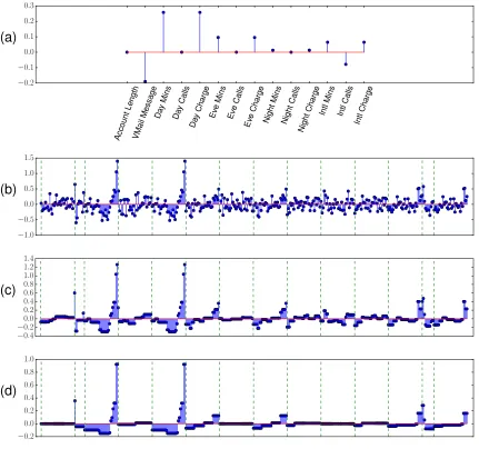
An important fact is that this optimization problem is numerically cheap, as explained in the next paragraph. Figure 1 illustrates the effect of the binarsity penalization with a varying strength on an example.

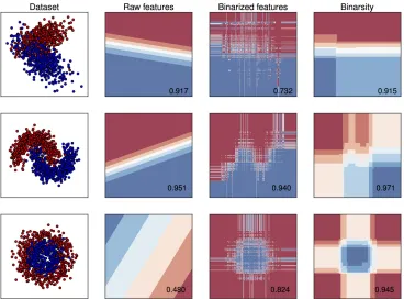
In Figure 2, we illustrate on a toy example, whenp = 2, the decision boundaries obtained for

logistic regression (LR) on raw features, LR on binarized features and LR on binarized features with the binarsity penalization.

Proximal operator of binarsity. The proximal operator and proximal algorithms are important tools for non-smooth convex optimization, with important applications in the field of supervised learning with structured sparsity (Bach et al., 2012). The proximal operator of a proper lower

semi-continuous (Bauschke and Combettes, 2011) convex functiong:Rd→Ris defined by

proxg(v)∈argminu∈Rd

n1

2kv−uk 2

2+g(u)

o .

Proximal operators can be interpreted as generalized projections. Namely, ifgis the indicator of a

convex setC _⊂Rdgiven by

g(u) =δC(u) = (

0 ifu_∈C,

∞ otherwise,

thenproxgis the projection operator ontoC. It turns out that the proximal operator of binarsity can

be computed very efficiently, using an algorithm (Condat, 2013) that we modify in order to include

weightswˆj,k. It applies in each group the proximal operator of the total-variation since binarsity

penalization is block separable, followed by a simple projection onto span(nj)⊥ the orthogonal

of span(nj), see Algorithm 1 below. We refer to Algorithm 2 in Section 6.2 for the weighted

total-variation proximal operator.

Proposition 1 Algorithm 1 computes the proximal operator ofbina(θ)given by(5).

(7)

Account Length

VMail Message Day

Mins Day

Calls

Day Charge

Eve Mins

Eve Calls

Eve Charge

Night Mins

Night Calls

Night Charge IntlMins Intl

Calls

Intl Charge −0.2

−0.1 0.0 0.1 0.2 0.3

(a)

−1.0

−0.5 0.0 0.5 1.0 1.5

(b)

−0.4

−00..20 0.2 0.4 0.6 0.8 1.0 1.2 1.4

(c)

−0.2 0.0 0.2 0.4 0.6 0.8 1.0

(d)

Fig. 1: Illustration of the binarsity penalization on the “Churn” dataset (see Section 4 for details) using

(8)

Fig. 2: Illustration of binarsity on 3 simulated toy datasets for binary classification with two classes (blue and red points). We set n = 1000, p = 2 andd1 = d2 = 100. In each row, we display the

simulated dataset, followed by the decision boundaries for a logistic regression classifier trained on initial raw features, then on binarized features without regularization, and finally on binarized features with binarsity. The corresponding testing AUC score is given on the lower right corner of each figure. Our approach allows to keep an almost linear decision boundary in the first row, while a good decision boundaries are learned on the two other examples, which correspond to non-linearly separable datasets, without apparent overfitting.

Algorithm 1:Proximal operator ofbina(θ), see (5)

Input:vectorθ_∈Rdand weightswˆj,kandnj,k forj= 1, . . . , pandk= 1, . . . , dj Output: vectorη= prox_bina(θ)

forj= 1topdo

βj,• ←proxkθj,•kTV,_wj,ˆ _•(θj,•)(TV-weighted prox in blockj, see (4))

ηj,• ←βj,•− n>_jβj,•

knjk22 nj (projection onto span(nj)

⊥₎

Return: η

3. Theoretical guarantees

We now investigate the statistical properties of (8) where the weights in the binarsity penalization have the form

ˆ

wj,k =O

r

logd n ˆπj,k

, with πˆj,k=

(9)

for allk_{∈ {}2, . . . , dj}, see Theorem 2 for a precise definition ofwˆj,k. Note thatπˆj,kcorresponds to

the proportion of ones in the sub-matrix obtained by deleting the firstkcolumns in thej-th binarized

block matrixXB•,j.In particular, we haveˆπj,k >0for allj, k. We consider the risk measure defined

by

R(mθ) =

1

n n X

i=1

−b0(m0(xi))mθ(xi) +b(mθ(xi)) ,

which is standard with generalized linear models (van de Geer, 2008).

3.1. A general oracle inequality

We aim at evaluating how “close” to the minimal possible expected risk our estimated functionm_θˆ

withθˆgiven by (8) is. To measure this closeness, we establish a non-asymptotic oracle inequality

with a fast rate of convergence considering the excess risk ofm_θˆ, namelyR(m_θˆ) −R(m0). To

derive this inequality, we consider for technical reasons the following problem instead of (7):

ˆ

θ_∈argmin_θ∈B_d₍_ρ₎

Rn(θ) + bina(θ) , (8)

where

Bd(ρ) = n

θ_∈Rd: p X

j=1

kθj,•k∞≤ρ

o .

This constraint is standard in literature for the proof of oracle inequalities for sparse generalized linear models, see for instance van de Geer (2008), and is discussed in details below.

We also impose a restricted eigenvalue assumption on XB. For all θ _∈ Rd, let J(θ) =

[J1(θ), . . . , Jp(θ)]be the concatenation of the support sets relative to the total-variation

penaliza-tion, that is

Jj(θ) ={k= 2, . . . , dj : θj,k 6=θj,k−1}.

Similarly, we denoteJ{₍_θ_{) =}

J{

1(θ), . . . , Jp{(θ)

the complementary ofJ(θ).The restricted

eigen-value condition is defined as follow.

Assumption 2 LetK = [K1, . . . , Kp]be a concatenation of index sets such that p

X

j=1

|Kj| ≤J?, (9)

whereJ?is a positive integer. Define

κ(K)_∈ inf

u∈_CTV,wˆ(K)\{0}

(

kXBu_k2

√

nkuKk2

)

with

CTV,wˆ(K) =

u_∈Rd: p X

j=1

k(uj,•)_K

j{kTV,wˆj,• ≤2 p X

j=1

k(uj,•)KjkTV,wˆj,•

. (10)

We assume that the following condition holds

κ(K)>0 (11)

(10)

The setCTV,wˆ(K)is a cone composed by all vectors with a support “close” toK. Theorem 2 gives

a risk bound for the estimatorm_θˆ.

Theorem 2 Let Assumptions 1 and 2 be satisfied. FixA >0and choose

ˆ

wj,k = r

2Unφ(A+ logd)

n πˆj,k. (12)

Then, with probability at least1₋2e−A, anyθˆgiven by(8)satisfies

R(m_θˆ)−R(m0)≤inf

θ n

3(R(mθ)−R(m0))

+2560(Cb(Cn+ρ) + 2)

Lnκ2(J(θ)) |

J(θ)_| max

j=1,...,pk( ˆwj,•)Jj(θ)k

2

∞ o

,

where the infimum is over the set of vectorsθ _∈ Bd(ρ)such thatn>j θj,• = 0for allj = 1, . . . , p and such that_|J(θ)| ≤J∗.

The proof of Theorem 2 is given in Section 6.3 below. Note that the “variance” term or “com-plexity” term in the oracle inequality satisfies

|J(θ)| max

2

∞≤2Unφ|

J(θ)|(A+ logd)

n . (13)

The value|J(θ)_|characterizes the sparsity of the vectorθ, given by

|J(θ)_|=

p X

j=1

|Jj(θ)|= p X

j=1

|{k= 1, . . . , dj :θj,k 6=θj,k−1}|.

It counts the number of non-equal consecutive values ofθ. Ifθis block-sparse, namely whenever

|J(θ)_|pwhereJ(θ) = _{j = 1, . . . , p:θj,• 6= 0dj}(meaning that few raw features are useful

for prediction), then|J(θ)| ≤ |J(θ)|maxj∈J(θ)|Jj(θ)|, which means that|J(θ)|is controlled by

the block sparsity_|J(θ)_|.

The oracle inequality from Theorem 2 is stated uniformly for vectors θ _∈ Bd(ρ) satisfying

n>_jθj,• = 0for allj = 1, . . . , pand|J(θ)| ≤J∗. Writing this oracle inequality under the

assump-tion _|J(θ)_{| ≤} J∗ meets the standard way of stating sparse oracle inequalities, see e.g. B¨uhlmann

and van De Geer (2011). Note thatJ∗is introduced in Assumption 2 and corresponds to a maximal

sparsity for which the matrixXB satisfies the restricted eigenvalue assumption. Also, the oracle

inequality stated in Theorem 2 stands for vectors such thatn>_j θj,• = 0, which is natural since the

binarsity penalization imposes these extra linear constraints.

The assumption that θ ∈ Bd(ρ) is a technical one, that allows to establish a connection, via

the notion of self-concordance, see Bach (2010), between the empirical squared`2-norm and the

empirical Kullback divergence (see Lemma 9 in Section 6.3). It corresponds to a technical constraint which is commonly used in literature for the proof of oracle inequalities for sparse generalized linear models, see for instance van de Geer (2008), a recent contribution for the particular case of Poisson regression being Ivanoff et al. (2016). Also, note that

max

i=1,...,n|hx B i , θi| ≤

p X

j=1

(11)

wherekθ_k∞= maxj=1,...,pkθj,•k∞. The first inequality in (14) comes from the fact that the entries

ofXBare in{0,1}, and it entails thatmaxi=1,...,n|hxBi , θi| ≤ρwheneverθ∈Bd(ρ). The second

inequality in (14) entails thatρcan be upper bounded by_|J(θ)_|×kθ_k∞, and therefore the constraint

θ_∈Bd(ρ)becomes only a box constraint onθ, which depends on the dimensionality of the features

through|J(θ)|only. The fact that the procedure depends onρ, and that the oracle inequality stated

in Theorem 2 depends linearly onρis commonly found in literature about sparse generalized linear

models, see van de Geer (2008); Bach (2010); Ivanoff et al. (2016). However, the constraintBd(ρ)

is a technicality which is not used in the numerical experiments provided in Section 4 below. In the next Section, we exhibit a consequence of Theorem 2, whenever one considers the

Gaus-sian case (least-squares loss) and where m0 has a sparse additive structure defined below. This

structure allows to control the bias term from Theorem 2 and to exhibit a convergence rate.

3.2. Sparse linear additive regression

Theorem 2 allows to study a particular case, namely an additive model, see e.g. Hastie and Tibshirani (1990); Horowitz et al. (2006) and in particular a sparse additive linear model, which is of particular interest in high-dimensional statistics, see Meier et al. (2009); Ravikumar et al. (2009); B¨uhlmann and van De Geer (2011). We prove in Theorem 3 below that our procedure matches the convergence rates previously known from literature. In this setting, we work under the following assumptions.

Assumption 3 We assume to simplify that xi ∈ [0,1]d for all i = 1, . . . , n. We consider the Gaussian setting with the least-squares loss, namely`(y, y0) = 1

2(y−y

0₎2_,_b₍_y_{) =} 1 2y

2_and_φ₌_σ2

(noise variance) in Equation(2), with Ln = Un = 1, Cb = 0in Assumption 1. Moreover, we assume thatm0has the following sparse additive structure

m0(x) = X

j∈J∗

m0_j(xj)

forx= [x1· · ·xp]∈Rp, wheremj0 :R→RareL-Lipschitz functions, namely satisfying|m0j(z)−

m0_j(z0)_{| ≤}L_|z₋z0_|for anyz, z0 _∈R, and whereJ∗ ⊂ {1, . . . , p}is a set of active features (sparsity means that_|J∗| p). Also, we assume the following identifiability condition

n X

i=1

m0_j(xi,j) = 0

for allj= 1, . . . , p.

Assumption 3 contains identifiability and smoothness requirements that are standard when

studying additive models, see e.g. Meier et al. (2009). We restrict the functionsm0_j to be

Lips-chitz and not smoother, since our procedure produces a piecewise constant decision function with

respect to eachj, that can approximate optimally only Lipschitz functions. For more regular

func-tions, our procedure would lead to suboptimal rates, see also the discussion below the statement of Theorem 3.

(12)

as in Theorem 2. Introduce alsoθ_j,k∗ = Pn

i=1m0j(xi,j)1Ik(xi,j)/ Pn

i=11Ik(xi,j) forj ∈ J∗ and θ∗_j,• =0Dforj /∈ J∗. Then, under Assumption 2 withJ∗ =J(θ∗)and Assumption 3, we have

km_θˆ−m0k2n≤

3L2|J∗|+5120Mnσ

2₍_A_{+ log(}_pn1/3_M

n) κ2₍_J₍_θ∗₎₎

|J_∗| n2/3,

whereMn= maxj=1,...,pmaxi=1,...,n|m0j(xi,j)|.

The proof of Theorem 3 is given in Section 6.8 below. It is an easy consequence of Theorem 2

under the sparse additive model assumption. It uses Assumption 2 withJ∗ = J(θ∗), sinceθ_j,•∗ is

the minimizer of the bias for eachj∈ J∗, see the proof of Theorem 3 for details.

The rate of convergence is, up to constants and logarithmic terms, of order_|J∗|2n−2/3.

Recall-ing that we work under a Lipschitz assumption, namely H¨older smoothness of order1, the scaling

of this rate w.r.t. to nis n−2r/(2r+1) with r = 1, which matches the one-dimensional minimax

rate. This rate matches the one obtained in B¨uhlmann and van De Geer (2011), see Chapter 8

p. 272, where the rate_|J∗|2n−2r/(2r+1) = |J∗|2n−4/5 is derived under aC2 smoothness

assump-tion, namelyr= 2. Hence, Theorem 3 shows that, in the particular case of a sparse additive model,

our procedure matches in terms of convergence rate the state of the art. Further improvements could consider more general smoothness (beyond Lipschitz) and adaptation with respect to the regularity, at the cost of a more complicated procedure which is beyond the scope of this paper.

4. Numerical experiments

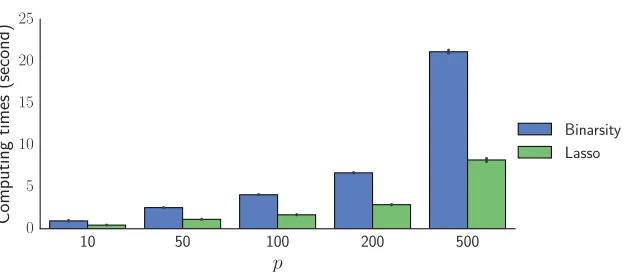
In this section, we first illustrate the fact that the binarsity penalization is roughly only two times

slower than basic`1-penalization, see the timings in Figure 3. We then compare binarsity to a large

number of baselines, see Table 2, using 9 classical binary classification datasets obtained from the UCI Machine Learning Repository (Lichman, 2013), see Table 3.

For each method, we randomly split all datasets into a training and a test set (30% for testing),

and all hyper-parameters are tuned on the training set usingV-fold cross-validation withV = 10.

For support vector machine with radial basis kernel (SVM), random forests (RF) and gradient

boost-ing (GB), we use the reference implementations from thescikit-learnlibrary (Pedregosa et al.,

2011), and we use theLogisticGAMprocedure from thepygamlibrary1for the GAM baseline.

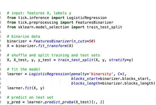
The binarsity penalization is proposed in thetick library (Bacry et al., 2018), we provide

sam-ple code for its use in Figure 4. Logistic regression with no penalization or ridge penalization gave similar or lower scores for all considered datasets, and are therefore not reported in our experiments.

The binarsity penalization does not require a careful tuning ofdj (number of bins for the

one-hot encoding of raw featurej). Indeed, past a large enough value, increasingdj even further barely

changes the results since the cut-points selected by the penalization do not change anymore. This

is illustrated in Figure 5, where we observe that past50 bins, increasingdj even further does not

affect the performance, and only leads to an increase of the training time. In all our experiments,

we therefore fixdj = 50forj= 1, . . . , p.

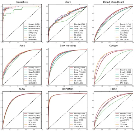
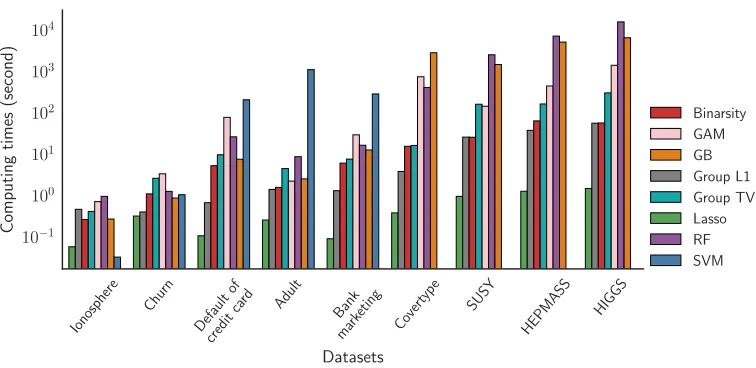
The results of all our experiments are reported in Figures 6 and 7. In Figure 6 we compare the performance of binarsity with the baselines on all 9 datasets, using ROC curves and the Area Under the Curve (AUC), while we report computing (training) timings in Figure 7. We observe that bina-rsity consistently outperforms Lasso, as well as Group L1: this highlights the importance of the TV

(13)

10 50 100 200 500 p

0 5 10 15 20 25

Computing

times

(second)

Binarsity Lasso

Fig. 3: Average computing time in second (with the black lines representing_±the standard deviation)

ob-tained on 100 simulated datasets for training a logistic model with binarsity VS Lasso penalization, both trained onXB withdj = 10for allj ∈1, . . . , p. Features are Gaussian with a Toeplitz

co-variance matrix with correlation0.5andn= 10000. Note that the computing time ratio between the two methods stays roughly constant and equal to2.

Name Description Reference

Lasso Logistic regression (LR) with`1penalization Tibshirani (1996b)

Group L1 LR with group`1penalization Meier et al. (2008)

Group TV LR with group total-variation penalization

SVM Support vector machine with radial basis kernel Sch¨olkopf and Smola (2002) GAM Generalized additive model Hastie and Tibshirani (1990)

RF Random forest classifier Breiman (2001)

GB Gradient boosting Friedman (2002)

Tab. 2: Baselines considered in our experiments. Note that Group L1 and Group TV are considered on

binarized features.

Dataset #Samples #Features Reference Ionosphere 351 34 Sigillito et al. (1989)

Churn 3333 21 Lichman (2013)

Default of credit card 30000 24 Yeh and Lien (2009)

Adult 32561 14 Kohavi (1996)

Bank marketing 45211 17 Moro et al. (2014) Covertype 550088 10 Blackard and Dean (1999)

SUSY 5000000 18 Baldi et al. (2014) HEPMASS 10500000 28 Baldi et al. (2016) HIGGS 11000000 24 Baldi et al. (2014)

(14)

Fig. 4: Sample python code for the use of binarsity with logistic regression in theticklibrary, with the use of theFeaturesBinarizertransformer for features binarization.

3 5 10 50 100 150 300 dj

0.74 0.76 0.78 0.80

AUC

AUC times dj= 50

0 10 20 30 40

Computing

times

(second)

Adult

3 5 10 50 100 150 300 dj

0.68 0.69 0.70 0.71

AUC

0 50 100

Computing

times

(second)

Default of credit card

Fig. 5: Impact of the number of bins used in each block (dj) on the classification performance (measured

by AUC) and on the training time using the “Adult” and “Default of credit card” datasets. Alldjare

equal forj = 1, . . . , p, and we consider in all cases the best hyper-parameters selected after cross validation. We observe that pastdj= 50bins, performance is roughly constant, while training time

(15)

0.0 0.2 0.4 0.6 0.8 1.0

0.0

0.2

0.4

0.6

0.8

1.0

Ionosphere

Binarsity (0.976) Group L1 (0.970) Group TV (0.972) Lasso (0.904) SVM (0.975) RF (0.980) GB (0.974) GAM (0.952)

0.0 0.2 0.4 0.6 0.8 1.0

0.0

0.2

0.4

0.6

0.8

1.0

Churn

0.0 0.2 0.4 0.6 0.8 1.0

0.0

0.2

0.4

0.6

0.8

1.0

Default of credit card

0.0 0.2 0.4 0.6 0.8 1.0

0.0

0.2

0.4

0.6

0.8

1.0

Adult

0.0 0.2 0.4 0.6 0.8 1.0

0.0

0.2

0.4

0.6

0.8

1.0

Bank marketing

0.0 0.2 0.4 0.6 0.8 1.0

0.0

0.2

0.4

0.6

0.8

1.0

Covtype

Binarsity (0.822) Group L1 (0.820) Group TV (0.821) Lasso (0.663) RF (0.863) GB (0.881) GAM (0.821)

0.0 0.2 0.4 0.6 0.8 1.0

0.0

0.2

0.4

0.6

0.8

1.0

SUSY

0.0 0.2 0.4 0.6 0.8 1.0

0.0

0.2

0.4

0.6

0.8

1.0

HEPMASS

0.0 0.2 0.4 0.6 0.8 1.0

0.0

0.2

0.4

0.6

0.8

1.0

HIGGS

Fig. 6: Performance comparison using ROC curves and AUC scores (given between parenthesis) computed

(16)

Ionosphere Churn

Default of

credit

card Adult _Bank

mark eting

Covert ype

SUSY

HEPMASS HIGGS

Datasets

10−1

100

101

102

103

104

Computing

times

(second)

Binarsity GAM GB Group L1 Group TV Lasso RF SVM

Fig. 7: Computing time comparisons (in seconds) between the methods on the considered datasets. Note

that the time values arelog-scaled. These timings concern the learning task for each model with the best hyper parameters selected, after the cross validation procedure. The 4 last datasets contain too many examples for the SVM with RBF kernel to be trained in a reasonable time. Roughly, binarsity is between 2 and 5 times slower than`1penalization on the considered datasets, but is more than 100

times faster than random forests or gradient boosting algorithms on large datasets, such as HIGGS.

norm within each group. The AUC of Group TV is always slightly below the one of binarsity, and more importantly it involves a much larger training time: convergence is slower for Group TV, since it does not use the linear constraint of binarsity, leading to a ill-conditioned problem (sum of binary features equals 1 in each block). Finally, binarsity outperforms also GAM and its performance is comparable in all considered examples to RF and GB, with computational timings that are orders of magnitude faster, see Figure 7. All these experiments illustrate that binarsity achieves an extremely competitive compromise between computational time and performance, compared to all considered baselines.

5. Conclusion

(17)

6. Proofs

In this Section we gather the proofs of all the theoretical results proposed in the paper. Throughout

this Section, we denote by∂(φ)the subdifferential mapping of a convex functionφ.

6.1. Proof of Proposition 1

Recall that the indicator function δj is given by (6). For any fixedj = 1, . . . , p, we prove that

prox_k·k_TV_,_ˆ

wj,•+δj is the composition ofproxk·kTV,wj,ˆ • andproxδj,namely

proxk·kTV,_wj,ˆ •+δj(θj,•) = proxδj proxk·kTV,_wj,ˆ •(θj,•)

for allθj,• ∈Rdj. Using Theorem 1 in Yu (2013), it is sufficient to show that for allθj,• ∈Rdj,we

have

∂ kθj,•kTV,wˆj,•

⊆∂ kprox_δ_j(θj,•)kTV,wˆj,•

. (15)

We have prox_δ_j(θj,•) = Πspan{nj}⊥(θj,•),whereΠspan{nj}⊥(·) stands for the projection onto the

orthogonal of span_{nj}. This projection simply writes

Π_span{n_j_}⊥(θj,•) =θj,•− n>_jθj,•

knjk2₂ nj

Now, let us define thedj ×dj matrixDj by

Dj = 

   

1 0 0

−1 1

. .. ...

0 −1 1



   

∈Rdj ×Rdj. (16)

We then remark that for allθj,•∈Rdj,

kθj,•kTV,wˆj,• =

dj X

k=2 ˆ

wj,k|θj,k−θj,k−1|=kwˆj,•Djθj,•k1. (17)

Using subdifferential calculus (see details in the proof of Proposition 5 below), one has

∂ _kθj,•kTV,wˆj,•

=∂ _kwˆj,•Djθj,•k1

=Dj>wˆj,•sign(Djθj,•).

Then, the linear constraintn>_jθj,•= 0entails

Dj>wˆj,•sign(Djθj,•) =Dj>wˆj,•sign

Dj θj,•− n>_j θj,•

knjk2₂ nj

,

(18)

6.2. Proximal operator of the weighted TV penalization

We recall in Algorithm 2 an algorithm provided in Alaya et al. (2015) for the computation of the proximal operator of the weighted total-variation penalization

β= proxk·kTV,wˆ(θ)∈argminθ∈Rm

n1

2kβ−θk 2

2+kθkTV,wˆ

o

. (18)

A quick explanation of this algorithm is as follows. The algorithm runs forwardly through the input

vector(θ1, . . . , θm).Using Karush-Kuhn-Tucker (KKT) optimality conditions (Boyd and

Vanden-berghe, 2004), we have that at a locationk,the weightβk stays constant whenever|uk|< wˆk+1,

whereuk is a solution to a dual problem associated to the primal problem (18). If not possible, it

goes back to the last location where a jump can be introduced inβ, validates the current segment

until this location, starts a new segment, and continues.

6.3. Proof of Theorem 2

The proof relies on several technical properties that are described below. From now on, we consider

y= [y1· · ·yn]>,X = [x1· · ·xn]>,m0(X) = [m0(x1)· · ·m0(xn)]>,and recalling thatmθ(xi) = θ>xB_i )we introducemθ(X) = [mθ(x1)· · ·mθ(xn)]>andb0(mθ(X)) = [b0(mθ(x1))· · ·b0(mθ(xn))]>.

Let us now define the Kullback-Leibler divergence between the true probability density funtion

f0defined in (2) and a candidatefθwithin the generalized linear modelfθ(y|x) = exp ymθ(x)−

b(mθ(x))as follows

KLn(f0, fθ) =

1

n n X

i=1

EPy|X

h

logf 0₍_y

i|xi) fθ(yi|xi) i

:= KLn(m0(X), mθ(X)),

wherePy|X is the joint distribution ofygivenX. We then have the following Lemma.

Lemma 4 The excess risk satisfies

R(mθ)−R(m0) =φKLn(m0(X), mθ(X)),

where we recall thatφis the dispertion parameter of the generalized linear model, see(2).

Proof.If follows from the following simple computation

KLn(m0(X), mθ(X))

=φ−11 n

n X

i=1

EPy|X

h

−yimθ(xi) +b(mθ(xi))

− −yim0(xi) +b(m0(xi))

i

=φ−1 R(mθ)−R(m0)

(19)

Algorithm 2:Proximal operator of weighted TV penalization

Input:vectorθ= θ1, . . . , θm >

∈Rmand weightswˆ= ( ˆw1, . . . ,wˆm)∈Rm+. Output: vectorβ = proxk·kTV,wˆ(θ)

1. Setk=k0=k− =k+←1

βmin←θ1−wˆ2; βmax←θ1+ ˆw2

umin←wˆ2; umax← −wˆ2

2. ifk=mthen

βm←βmin+umin

3. ifθk+1+umin< βmin−wˆk+2then /* negative jump */

βk0 =· · ·=βk− ←βmin k=k0=k−=k+←k−+ 1

βmin←θk−wˆk+1+ ˆwk; βmax←θk+ ˆwk+1+ ˆwk

umin←wˆk+1; umax← −wˆk+1

4. else ifθk+1+umax> βmax+ ˆwk+2then /* positive jump */

βk0 =. . .=βk+←βmax

k=k0=k−=k+←k++ 1

βmin←θk−wˆk+1−wˆk; βmax←θk+ ˆwk+1−wˆk

umin←wˆk+1; umax← −wˆk+1

5. else _{/* no jump */}

setk_←k+ 1

umin←θk+ ˆwk+1−βmin

umax←θk−wˆk+1−βmaxifumin≥wˆk+1then

βmin←βmin+

umin−wˆk+1

k−k0+1

umin←wˆk+1

k− ←k

ifumax≤ −wˆk+1then

βmax←βmax+

umax+ ˆwk+1

k−k0+1

umax← −wˆk+1

k+ ←k

6. ifk < mthen go to3.

7. ifumin<0then

βk0 =· · ·=βk− ←βmin k=k0=k−←k−+ 1 βmin←θk−wˆk+1+ ˆwk

umin←wˆk+1; umax←θk+ ˆwk−vmax

go to2.

8. else ifumax>0then

βk0 =· · ·=βk+←βmax

k=k0=k+←k++ 1

βmax←θk+ ˆwk+1−wˆk

umax← −wˆk+1; umin←θk−wˆk−umin

go to2.

9. else

βk0 =· · ·=βm←βmin+

umin

(20)

6.4. Optimality conditions

As explained in the following Proposition, a solution to problem (8) can be characterized using the Karush-Kuhn-Tucker (KKT) optimality conditions (Boyd and Vandenberghe, 2004).

Proposition 5 A vector θˆ = [ˆθ>₁_,•· · ·θˆ>p,•]> ∈ Rd is an optimum of the objective function (8) if and only if there are subgradients ˆh = [ˆhj,•]j=1,...,p ∈ ∂kθˆkTV,wˆ and gˆ = [ˆgj,•]j=1,...,p ∈ ∂[δj(ˆθj,•)]j=1,...,psuch that

∇Rn(ˆθj,•) + ˆhj,•+ ˆgj,•=0, where

(

ˆ

hj,• =D>_j wˆj,•sign(Djθˆj,•) ifj∈J(ˆθ),

ˆ

hj,• ∈D>_j wˆj,•[−1,+1]dj

ifj_∈J{(ˆθ), (19)

and where we recall thatJ(ˆθ)is the support set ofθ. The subgradientˆ gˆj,•belongs to

∂ δj(ˆθj,•)=µj,•∈Rdj :µ>j,•θj,• ≤µ>j,•θˆj,• for all θj,• such that n>jθj,•= 0 . For the generalized linear model, we have

1

n X B •,j

>

b0(m_θˆ(X))−y

+ ˆhj,•+ ˆgj,•+ ˆfj,• =0, (20)

wherefˆ= [ ˆfj,•]j=1,...,pbelongs to the normal cone of the ballBd(ρ).

Proof.The functionθ_7→Rn(θ)is differentiable, so the subdifferential ofRn(·) + bina(·)at a point θ= (θj,•)j=1,...,p∈Rdis given by

∂(Rn(θ) + bina(θ)) =∇Rn(θ) +∂(bina(θ)),

where_∇Rn(θ) =

h_∂R n(θ) ∂θ1,• · · ·

∂Rn(θ) ∂θp,•

i>

and

∂bina(θ) =h∂_kθ1,•kTV,wˆ1,•+∂δj(θ1,•) · · · ∂kθp,•kTV,wˆp,•+∂δj(θp,•)

i> .

We have_kθj,•kTV,wˆj,• =kwˆj,•Djθj,•k1for allj= 1, . . . , p. Then, by applying some properties

of the subdifferential calculus, we get

∂_kθj,•kTV,wˆj,• =

(

D_j>sign( ˆwj,•Djθj,•) ifDjθ6=0,

D_j> wˆj,•vj) otherwise,

(21)

wherevj ∈[−1,+1]dj for allj= 1, . . . , p. For generalized linear models, we rewrite

ˆ

θ∈argminθ∈Rd

Rn(θ) + bina(θ) +δBd(ρ)(θ) , (22)

whereδBd(ρ)is the indicator function ofBd(ρ). Now,θˆ= [ˆθ

>

1,•· · ·θˆp,•> ]>is an optimum of (22) if

and only if0_{∈ ∇}Rn(m_θˆ) +∂kθˆkTV,wˆ+∂δBd(ρ)(ˆθ). Recall that the subdifferential ofδBd(ρ)(·)is

the normal cone ofBd(ρ), namely

∂δBd(ρ)(ˆθ) =

η ∈Rd:η>θ≤η>θˆfor allθ∈Bd(ρ)}. (23)

One has

∂Rn(θ) ∂θj,•

= 1

n(X B

•,j)>(b0(m_θˆ(X))−y), (24)

(21)

6.5. Compatibility conditions

Let us define the block diagonal matrixD= diag(D1, . . . , Dp)withDj defined in (16). We denote

its inverseTj which is defined by thedj ×dj lower triangular matrix with entries(Tj)r,s = 0if

r < sand(Tj)r,s= 1otherwise. We setT= diag(T1, . . . , Tp), so that one hasD−1 =T.

In order to prove Theorem 2, we need the following results which give a compatibility

prop-erty (van de Geer, 2008; van de Geer and Lederer, 2013; Dalalyan et al., 2017) for the matrixT, see

Lemma 6 below and for the matrixXBT, see Lemma 7 below. For any concatenation of subsets

K = [K1, . . . , Kp],we set

Kj ={τj1, . . . , τ bj

j } ⊂ {1, . . . , dj} (25)

for allj= 1, . . . , pwith the convention thatτ_j0= 0andτbj+1

j =dj + 1.

Lemma 6 Letγ ∈Rd+be given andK = [K1, . . . , Kp]withKjgiven by(25)for allj= 1, . . . , p. Then, for everyu_∈Rd\{0}, we have

kTu_k2

|kuKγKk1− ku_K{ γ_K{k1| ≥

κT,γ(K),

where

κT,γ(K) =

32

p X

j=1

dj X

k=1

|γj,k+1−γj,k|2+ 2|Kj|kγj,•k2∞∆−min1,Kj −1/2

,

and∆min,Kj = minr=1,...bj|τ_jrj−τrj −1

j |.

Proof.Using Proposition 3 in Dalalyan et al. (2017), we have

kuKγKk1− ku_K{ γ_K{k1

=

p X

j=1

kuKj γKjk1− ku_K_j{ γ_K

j{k1

≤

p X

j=1

4_kTjuj,•k2

2

dj X

k=1

|γj,k+1−γj,k|2+ 2(bj+ 1)kγj,•k2∞∆−min1,Kj 1/2

.

Using H¨older’s inequality for the right hand side of the last inequality gives

kuKγKk1− ku_K{ γ_K{k1

≤ kTu_k2

32

p X

j=1

dj X

k=1

|γj,k+1−γj,k|2+ 2|Kj|kγj,•k2∞∆−min1,Kj 1/2

,

which completes the proof of the Lemma.

Combining Assumption 2 and Lemma 6 allows to establish a compatibility condition satisfied

(22)

Lemma 7 Letγ _∈ Rd+ be given andK = [K1, . . . , Kp]withKj given by(25)forj = 1, . . . , p. Then, if Assumption 2 holds, one has

inf

u∈_C1,wˆ(K)\{0}

n kXBTuk₂

√

n_{| k}uKγKk1− kuK{ γ_K{k1|

o

≥κT,γ(K)κ(K), (26)

where

C1,wˆ(K) =

n

u_∈Rd: p X

j=1

k(uj,•)_K

j{k1,wˆj,• ≤2 p X

j=1

k(uj,•)Kjk1,wˆj,•

o

. (27)

Proof.Lemma 6 gives

kXBTu_k2

√

n_|kuKγKk1− ku_K{γ_K{k1| ≥

κT,γ(K)k

XBTuk2 √

n_kTu_k2

.

Now, we note that ifu_∈C1,wˆ(K), thenTu∈CTV,wˆ(K).Hence, Assumption 2 entails

kXBTu_k2

√

n_|kuKγKk1− ku_K{γ_K{k1| ≥

κT,γ(K)κ(K),

which concludes the proof of the Lemma.

6.6. Connection between the empirical Kullback-Leibler divergence and the empirical squared norm

The next Lemma is from Bach (2010) (see Lemma 1 herein).

Lemma 8 Letϕ: R→ Rbe a three times differentiable convex function such that for allt ∈ R,

|ϕ000(t)_{| ≤}M_|ϕ00(t)_|for someM _≥0.Then, for allt_≥0, one has

ϕ00(0)

M2 ψ(−M t)≤ϕ(t)−ϕ(0)−ϕ

0₍₀₎_t

≤ ϕ

00₍₀₎

M2 ψ(M t),

withψ(u) =eu−u−1.

This Lemma entails the following in our setting.

Lemma 9 Under Assumption 1, one has

Lnψ(−2(Cn+ρ))

4φ(Cn+ρ)2

1

nkm

0₍_X₎₋_m

θ(X)k22 ≤KLn(m0(X), mθ(X)), Unψ(2(Cn+ρ))

4φ(Cn+ρ)2

1

nkm

0₍_X₎₋_m

θ(X)k22 ≥KLn(m0(X), mθ(X)),

for allθ_∈Bd(ρ).

Proof. Let us consider the functionGn:R→Rdefined byGn(t) = Rn(m0+tmη), withmη to

be defined later, which writes

Gn(t) =

1

n n X

i=1

b(m0(xi) +tmη(xi))−

1

n n X

i=1

(23)

We have

G0_n(t) = 1

n n X

i=1

mη(xi)b0(m0(xi) +tmη(xi))−

1

n n X

i=1

yimη(xi),

G00_n(t) = 1

n n X

i=1

m2_η(xi)b00(m0(xi) +tmη(xi)),

and G000_n(t) = 1

n n X

i=1

m3_η(xi)b000(m0(xi) +tmη(xi)).

Using Assumption 1, we have|G000_n(t)| ≤ Cbkmηk∞|G00_n(t)|wherekmηk∞ := max

i=1,...,n|mη(xi)|.

Lemma 8 withM =Cbkmηk∞gives

G00_n(0)ψ(−Cbkmηk∞t)

C2

bkmηk2∞

≤Gn(t)−Gn(0)−tG0n(0)≤G

00 n(0)

ψ(Cbkmηk∞t) C2

bkmηk2∞

for allt_≥0andt= 1leads to

G00_n(0)ψ(−Cbkmηk∞)

C_b2kmηk2∞ ≤

Rn(m0+mη)−Rn(m0)−G0n(0)≤G00n(0)

ψ(Cbkmηk∞) C_b2kmηk2∞

.

An easy computation gives

−G0_n(0) = 1

n n X

i=1

mη(xi) yi−b0(m0(xi))

and G00_n(0) = 1

n n X

i=1

m2_η(xi)b00(mη(xi)),

and since obviouslyEPy|X[G

0

n(0)] = 0, we obtain

G00_n(0)ψ(−Cbkmηk∞)

C_b2_kmηk2∞ ≤

R(m0+mη)−R(m0)≤G00n(0)

ψ(Cbkmηk∞) C_b2_kmηk2∞

.

Now, choosingmη =mθ−m0and combining Assumption 1 with Equation (14) gives

Cbkmηk∞≤Cb max i=1,...,n(|hx

B

i , θi|+|m0(xi)|)≤Cb(ρ+Cn).

Hence, sincex_7→ψ(x)/x2 is an increasing function onR+, we end up with

G00_n(0)ψ(−Cb(Cn+ρ))

C_b2(Cn+ρ)2 ≤

G00_n(0)ψ(Cb(Cn+ρ))

C_b2(Cn+ρ)2 ≥

and sinceG00_n(0) =n−1Pn

i=1(mθ(xi)−m0(xi))2b00(m0(xi)), we obtain Lnψ(−Cb(Cn+ρ))

C2

nφ(Cn+ρ)2

1

nkm

0₍_X₎

−mθ(X)k22 ≤KLn(m0(X), mθ(X)),

Unψ(Cb(Cn+ρ)) C_b2φ(Cn+ρ)2

1

nkm

0₍_X₎₋_m

θ(X)k22 ≥KLn(m0(X), mθ(X)),

(24)

Let us recall that

Rn(mθ) =

1

n n X

i=1

b(mθ(xi))−

1

n n X

i=1

yimθ(xi)

for allθ_∈Rdand that

ˆ

θ∈argminθ∈Bd(ρ)

Rn(θ) + bina(θ) . (28)

Proposition 5 above entails that there is ˆh = [ˆhj,•]j=1,...,p ∈ ∂kθˆkTV,wˆ, gˆ = [ˆgj,•]j=1,···,p ∈

[∂δj(ˆθj,•)]j=1,...,pandfˆ= [ ˆfj,•]j=1,...,p∈∂δBd(ρ)(ˆθ)such that

D1

n(X

B₎>₍_b0₍_m

ˆ

θ(X))−y) + ˆh+ ˆg+ ˆf ,θˆ−θ E

= 0

for allθ_∈Rd. This can be rewritten as

1

nhb 0₍_m

ˆ

θ(X))−b

0₍_m0₍_X₎₎_{, m} ˆ

θ(X)−mθ(X)i

−_n1hy₋b0(m0(X)), m_θˆ(X)−mθ(X)i+hˆh+ ˆg+ ˆf ,θˆ−θi= 0.

For any θ _∈ Bd(ρ) such that n>jθj,• = 0 for all j and h ∈ ∂kθkTV,wˆ, the monotony of the

subdifferential mapping implieshh, θˆ −θî ≤ hh, θ−θî,hg, θˆ −θî ≤0,andhf , θˆ −θî ≤0, so that

1

nhb 0₍_m

ˆ

θ(X))−b

0₍_m0₍_X₎₎_{, m} ˆ

θ(X)−mθ(X)i

≤ _n1hy₋b0(m0(X)), m_θˆ(X)−mθ(X)i − hh,θˆ−θi.

(29)

Now, consider the functionHn:R→Rdefined by

Hn(t) =

1

n n X

i=1

b(m_θˆ₊_tη(xi))−

1

n n X

i=1

b0(m0(xi))m_θˆ₊_tη(xi),

whereη will be defined later. We use again the same arguments as in the proof of Lemma 9. We

differentiateHnthree times with respectt, so that

H_n0(t) = 1

n n X

i=1

mη(xi)b0(m_θˆ₊_tη(xi))−

1

n n X

i=1

b0(m0(xi))mη(xi),

H_n00(t) = 1

n n X

i=1

m2_η(xi)b00(m_θˆ₊_tη(xi)),

and H_n000(t) = 1

n n X

i=1

m3_η(xi)b000(m_θˆ₊_tη(xi)),

and in the way as in the proof of Lemma 9, we have|H_n000(t)| ≤Cb(Cn+ρ)|Hn00(t)|, and Lemma 8

entails

H_n00(0)ψ(−Cbt(Cn+ρ))

C_b2(Cn+ρ)2 ≤

Hn(t)−Hn(0)−tHn0(0)≤Hn00(0)

ψ(Cbt(Cn+ρ)) C_b2(Cn+ρ)2

(25)

for allt_≥0. Takingt= 1andη=θ₋θˆimplies

Hn(1) =

1

n n X

i=1

b(mθ(xi))−

1

n n X

i=1

b0(m0(xi))mθ(xi) =R(mθ),

and Hn(0) =

1

n n X

i=1

b(m_θˆ(xi))−

1

n n X

i=1

b0(m0(xi))m_θˆ(xi) =R(m_θˆ).

Moreover, we have

H_n0(0) = 1

n n X

i=1

hxB_i , θ₋θˆ_ib0(m_θˆ(xi))−

1

n n X

i=1

b0(m0(xi))hxBi ,θˆ−θi

= 1

nhb 0₍_m

ˆ

θ(X))−b

0₍_m0₍_X₎₎_,_XB₍_θ

−θˆ)_i,

and H_n00(0) = 1

n n X

i=1

hxB_i ,θˆ₋θ_i2b00(m_θˆ(xi)).

Then, we deduce that

H_n00(0)ψ(−Cb(Cn+ρ))

C_b2(Cn+ρ)2 ≤

R(mθ)−R(m_θˆ)− 1

nhb 0₍_m

ˆ

θ(X))−b

0₍_m0₍_X₎₎_,_XB₍_θ

−θˆ)_i

=φKLn(m0(X), mθ(X))−φKLn(m0(X), m_θˆ(X))

+ 1

nhb 0₍_m

ˆ

θ(X))−b

0₍_m0₍_X₎₎_{, m} ˆ

θ(X)−mθ(X)i.

Then, with Equation (29), one has

φKLn(m0(X), m_θˆ(X)) +Hn00(0)

ψ(−Cb(Cn+ρ)) C2

b(Cn+ρ)2

≤φKLn(m0(X), mθ(X)) +

1

nhy−b

0₍_m0₍_X₎₎_{, m} ˆ

θ(X)−mθ(X)i − hh,θˆ−θi.

(30)

AsH_n00(0)_≥0, it implies that

φKLn(m0(X), m_θˆ(X))≤φKLn(m0(X), mθ(X))

+ 1

nhy−b

0₍_m0₍_X₎₎_{, m} ˆ

θ(X)−mθ(X)i − hh,θˆ−θi. (31)

If 1_n_hy₋b0(m0(X)),XB(ˆθ₋θ)_{i − h}h,θˆ₋θ_i<0,it follows that

KLn(m0(X), m_θˆ(X))≤KLn(m0(X), mθ(X)),

then Theorem 2 holds. From now on, let us assume that

1

nhy−b

0₍_m0₍_X₎₎_{, m} ˆ

(26)

We first derive a bound on _n1hy₋b0(m0(X)), m_θˆ(X)−mθ(X)i.Recall that D−1 = T (see

beginning of Section 6.5). We focus on finding out a bound for_n1h(XBT)>₍_y₋_b0₍_m0₍_X₎₎₎_,_D_(ˆ_θ₋

θ)i.On the one hand, one has

1

nh(X B₎>

(y−b0(m0(X))),θˆ−θi

= 1

nh(X B_T₎>

(y−b0(m0(X))),D(ˆθ−θ)i

≤ _n1

p X

j=1

dj

X

k=1

|((XB•,jTj)•,k)>(y−b0(m0(X)))| |(Dj(ˆθj,•−θj,•))k|

where (XB•,jTj)•,k = [(XB•,jTj)1,k· · ·(XB•,jTj)n,k]> ∈ Rn is the k-th column of the matrix

XB_•,jTj.Let us consider the event

En=

p \

j=1

dj \

k=2

En,j,k, whereEn,j,k= n1

n|(X B

•,jTj)>•,k(y−b0(m0(X)))| ≤wˆj,k o

,

so that, onEn, we have

1

nh(X B₎>₍_y

−b0(m0(X)),θˆ₋θ_{i ≤}

p X

j=1

dj X

k=1 ˆ

wj,k|(Dj(ˆθj,•−θj,•))k|

≤

p X

j=1

kwˆj,•Dj(ˆθj,•−θj,•)k1. (33)

On the other hand, from the definition of the subgradient [hj,•]j=1,...,p ∈ ∂kθkTV,wˆ (see

Equa-tion (19)), one can choosehsuch that

hj,k = (D>j ( ˆwj,•sign(Djθj,•)))k

for allk_∈Jj(θ)and

hj,k = (Dj>( ˆwj,•sign(Djθˆj,•))k= (D>j ( ˆwj,•sign(Dj(ˆθj,•−θj,•)))k

for allk∈J_j{(θ). Using a triangle inequality and the fact thatsign(x)>x=kxk1, we obtain

−hh,θˆ₋θ_{i ≤}

p X

j=1

k( ˆwj,•)Jj(θ)Dj(ˆθj,•−θj,•)Jj(θ)k1

−

p X

j=1

k( ˆwj,•)_J{

j(θ)Dj(ˆθj,•−θj,•)Jj{(θ)k1

≤

p X

j=1

k(ˆθj,•−θj,•)Jj(θ)kTV,wˆj,•−

p X

j=1

k(ˆθj,•−θj,•)_J{

(27)

Combining inequalities (33) and (34), we get

p X

j=1

k(ˆθj,•−θj,•)_J{

j(θ)kTV,wˆj,• ≤2 p X

j=1

k(ˆθj,•−θj,•)Jj(θ)kTV,wˆj,•

on_En. Hence

p X

j=1

k( ˆwj,•)_J{

j(θ)Dj(ˆθj,•−θj,•)Jj{(θ)k1≤2 p X

j=1

k( ˆwj,•)Jj(θ)Dj(ˆθj,•−θj,•)Jj(θ)k1.

This means that

ˆ

θ₋θ_∈CTV,wˆ(J(θ))andD(ˆθ−θ)∈C1,wˆ(J(θ)), (35)

see (10) and (27). Now, going back to (31) and taking into account (35), the compatibility ofXBT

given in Equation (26) provides the following on the eventEn:

φKLn(m0(X), m_θˆ(X))≤φKLn(m0(X), mθ(X))

+ 2

p X

j=1

k( ˆwj,•)Jj(θ)Dj(ˆθj,•−θj,•)Jj(θ)k1.

Then

KLn(m0(X), m_θˆ(X))≤KLn(m0(X), mθ(X)) + k

m_θˆ(X)−mθ(X)k2 √

n φ κT,ˆγ(J(θ))κ(J(θ))

, (36)

whereγˆ= (ˆγ₁>_,•, . . . ,γˆp,•> )>is such that

ˆ

γj,k =

2 ˆwj,k ifk∈Jj(θ),

0 ifk∈J_j{(θ),

for allj= 1, . . . , pand

κT,γˆ(J(θ)) =

32

p X

j=1

dj X

k=1

|γˆj,k+1−γˆj,k|2+ 2|Jj(θ)|kγˆj,•k2∞∆−_min1_,J_j₍_θ₎ −1/2

.

Now, we find an upper bound for

1

κ2

T,γˆ(J(θ)) = 32

p X

j=1

dj X

k=1

|ˆγj,k+1−ˆγj,k|2+ 2|Jj(θ)|kγˆj,•k2∞∆_min−1 _,J_j₍_θ₎.

Note thatkγˆj,•k∞≤2kwˆj,•k∞. Let us writeJj(θ) =

k_j1, . . . , k|J_j j(θ)| and setBr= [[kr−_j 1, kjr[[ =

(28)

k|Jj(θ)|+1

j =dj + 1. Then

dj X

k=1

|ˆγj,k+1−ˆγj,k|2 =

|Jj(θ)|+1 X

r=1

X

k∈Br

|γˆj,k+1−γˆj,k|2

=

|Jj(θ)|+1 X

r=1

|ˆγ_j,kr−1

j +1−γˆj,k r−1

j |

2₊ |γˆj,kr

j −γˆj,krj−1|

2

=

|Jj(θ)|+1 X

r=1 ˆ

γ_j,k2 r−1

j

+ ˆγ_j,k2 r j

=

|Jj(θ)| X

r=1

2 ˆγ_j,k2 r j

≤8_|Jj(θ)| k( ˆwj,•)Jj(θ)k

2

∞.

Therefore

1

κ2

T,ˆγ(J(θ))

≤512

p X

j=1

|Jj(θ)| k( ˆwj,•)Jj(θ)k

2

∞+|Jj(θ)| k( ˆwj,•)Jj(θ)k

2

∞∆−_min1 _,J_j₍_θ₎ ≤512 p X j=1

1 + 1

∆min,Jj(θ)

|Jj(θ)|k( ˆwj,•)Jj(θ)k

2

∞

≤512_|J(θ)_| max

2

∞.

(37)

Now, we use the connection between the empirical norm and Kullback-Leibler divergence. Indeed, using Lemma 9, we get

km_θˆ(X)−mθ(X)k2

√

nφκT,ˆγ(J(θ))κ(J(θ))

≤ √ 1

φκT,γˆ(J(θ))κ(J(θ))

1

√

nkmθˆ(X)−m

0₍_X₎_k 2+

1

√

nkm

0₍_X₎₋_m

θ(X)k2

≤ √ 2

φκT,γˆ(J(θ))κ(J(θ))

p

Cn(ρ, Ln)

KLn(m0(X), m_θˆ(X))1/2

+ KLn(m0(X), mθ(X))1/2

,

where we definedCn(ρ, Ln) = Ln_Cψ(2−Cb(Cn+ρ))

bφ(Cn+ρ)2 , so that combined with Equation (36), we obtain

KLn(m0(X), m_θˆ(X))≤KLn(m0(X), mθ(X))

+_√ 2

φκT,ˆγ(J(θ))κ(J(θ)) p

Cn(ρ, Ln)

KLn(m0(X), m_θˆ(X))1/2

+ KLn(m0(X), mθ(X))1/2

(29)

This inequality entails the following upper bound

KLn(m0(X), m_θˆ(X))≤3KLn(m0(X), mθ(X)) +

5

φκ2

T,ˆγ(J(θ))κ2(J(θ))Cn(ρ, Ln) ,

since whenever we have x _≤ c +b√x for some x, b, c > 0, then x _≤ 2c+b2_{. Introducing}

g(x) =x2/ψ(−x) =x2/(e−x+ 1−x), we note that

1

Cn(ρ, Ln)

= φ

Ln

g(Cb(Cn+ρ))≤ φ Ln

(Cb(Cn+ρ) + 2),

sinceg(x)_≤x+ 2for anyx >0. Finally, by using also (37), we end up with

KLn(m0(X), m_θˆ(X))≤3KLn(m0(X), mθ(X))+

2560(Cb(Cn+ρ) + 2) Lnκ2(J(θ)) |

J(θ)| k( ˆwj,•)Jj(θ)k

2

∞,

which is the statement provided in Theorem 2. The only thing remaining is to control the probability

of the eventE{

n. This is given by the following:

P[_E_n{]_≤

p X j=1 dj X k=2 P h1

n|(X B

•,jTj)>•,k(y−b0(m0(X)))| ≥wˆj,k i ≤ p X j=1 dj X k=2 Ph n X i=1

|(XB•,jTj)i,k(yi−b0(m0(xi)))| ≥nwˆj,k i

.

Let ξi,j,k = (XB•,jTj)i,k and Zi = yi −b0(m0(xi)).Note that conditionally on xi, the random

variables(Zi)are independent. It can be easily shown (see Theorem 5.10 in Lehmann and Casella

(1998)) that the moment generating function ofZ (copy ofZi) is given by

E[exp(tZ)] = exp(φ−1_{b(m0(x) +t)₋tb0(m0(x)₋b(m0(x)))_}). (38)

Applying Lemma 6.1 in Rigollet (2012), using (38) and Assumption 1, we can derive the following Chernoff-type bounds

Ph

n X

i=1

|ξi,j,kZi| ≥nwˆj,k i

≤2 exp₋ n 2_w_ˆ2

j,k

2Unφkξ•,j,kk22

, (39)

whereξ•,j,k= [ξ1,j,k· · ·ξn,j,k]>∈Rn.We have

XB_•,jTj = 

  

1 Pdj k=2xB1,j,k

Pdj

k=3xB1,j,k · · · Pdj

k=dj−1x

B

1,j,k xB1,j,dj

..

. ... ... ... ...

1 Pdj

k=2xBn,j,k Pdj

k=3xBn,j,k · · · Pdj

k=dj−1x

B

n,j,k xBn,j,dj     , therefore

kξ•,j,kk22=

n X

i=1

(XB_•,jTj)2•,k = # n

i:xi,j ∈ dj [

r=k Ij,r

o

=nπˆj,k. (40)

So, using the weightswˆj,k given by (12) together with (39) and (40), we obtain that the probability

(30)

First, let us note that in the least squares setting, we haveR(mθ)−R(m0) = kmθ −m0k2n for

any θ ∈ Rd where kgk2n = n1

Pn

i=1g(xi)2, and that b(y) = 1₂y2, φ = σ2 (noise variance) in

Equation (2), andLn=Un= 1,Cb = 0. Theorem 2 provides

km_θˆ−m0k2n≤3kmθ−mθ0k2_n+

5120σ2 κ2₍_J₍_θ₎₎

|J(θ)|(A+ logd)

n

for anyθ_∈ Rdsuch thatn>j θj• = 0andJ(θ) ≤ J∗. Sincedj = Dfor allj = 1, . . . , p, we have

d=Dpand

|J(θ)_|=

p X

j=1

|{k= 2, . . . , D:θj,k6=θj,k−1}| ≤(D−1)|J(θ)|kθk∞≤Dpkθk∞ (41)

for any θ ∈ Rd, where we recall that J(θ) = {j = 1, . . . , p : θj,• 6= 0D}. Also, recall that

Ij,1=I1 = [0,_D1]andIj,k =Ik = (k−_D1,_Dk]fork= 2, . . . , Dandj= 1, . . . , p. Also, we consider

θ=θ∗, whereθ_j,•∗ is defined, for anyj_{∈ J}∗, as the minimizer of

n X

i=1

XD

k=1

(θj,k−m0j(xi,j))1Ik(xi,j) 2

over the set of vectorsθj,• ∈RD satisfyingn>jθj,•= 0, and we putθ

∗

j,•=0Dforj /∈ J∗. It is easy

to see that the solution is given by

θ∗_j,k=

Pn

i=1m0j(xi,j)1Ik(xi,j) nj,k

,

where we recall thatnj,k =

Pn

i=11Ik(xi,j). Note in particular that the identifiability assumption

Pn

i=1m0j(xi,j) = 0entails thatn>j θ∗j,• = 0. In order to control the bias term, an easy computation

gives that, wheneverxi,j ∈Ik

|θ∗_j,k₋m0_j(xi,j)| ≤ Pn

i0₌₁|m0_j(xi0_,j)−m0_j(x_i,j)|1_I

k(xi0,j)

nj,k ≤

(31)

where we used the fact thatm0_j isL-Lipschitz, so that

kmθ∗−m0k2

n=

1

n n X

i=1

(mθ∗(x_i,j)−m0(x_i,j))2

= 1

n n X

i=1

X

j∈J∗

D X

k=1

(θ∗_j,k₋m0(xi,j))1Ik 2

≤ |J_n∗|

n X

i=1

X

j∈J∗

D X

k=1

(θ∗_j,k₋m0(xi,j))1Ik 2

≤ |J_n∗|

n X

i=1

X

j∈J∗

D X

k=1

(θ_j,k∗ ₋m0(xi,j))21Ik(xi,j)

≤ |J∗|

X

j∈J∗

D X

k=1

L2_|Ik|21Ik(xi,j)≤

L2_|J∗|2 D2 .

Note that|θ_j,k∗ | ≤ km0_jkn,∞wherekm0jkn,∞= maxi=1,...,n|m0j(xi,j)|. This entails thatkθ∗k∞≤

maxj=1,...,pkm0jkn,∞=Mn. So, using also (41), we end up with

km_θˆ−m0k2n≤

3L2|J∗|2

D2 +

5120σ2 κ2₍_J₍_θ∗₎₎

D_J∗Mn(A+ log(DpMn))

n ,

which concludes the proof Theorem 3 usingD=n1/3.

References

A. Agresti. Foundations of Linear and Generalized Linear Models. John Wiley & Sons, 2015.

M. Z. Alaya, S. Ga¨ıffas, and A. Guilloux. Learning the intensity of time events with change-points.

Information Theory, IEEE Transactions on, 61(9):5148–5171, 2015.

F. Bach. Self-concordant analysis for logistic regression.Electron. J. Statist., 4:384–414, 2010.

F. Bach, R. Jenatton, J. Mairal, and G. Obozinski. Optimization with sparsity-inducing penalties.

Foundations and TrendsR in Machine Learning, 4(1):1–106, 2012.

E. Bacry, M Bompaire, P. Deegan, S. Ga¨ıffas, and S. V. Poulsen. tick: a python library for statistical

learning, with an emphasis on hawkes processes and time-dependent models.Journal of Machine

Learning Research, 18(214):1–5, 2018. URLhttp://jmlr.org/papers/v18/17-381. html.

P. Baldi, P. Sadowski, and D. Whiteson. Searching for exotic particles in high-energy physics with

deep learning. Nature communications, 5, 2014.

P. Baldi, K. Cranmer, T. Faucett, P. Sadowski, and D. Whiteson. Parameterized neural networks for