ISSN: 2231-5373 http://www.ijmttjournal.org Page 304
Fuzzy Finite Element Method Applied To
Euler-Bernoulli Beam Problem
Deb Kumar Ranjit 1, Tapan Kumar Roy2
Department of Mathematics
Indian Institute of Engineering Science and Technology, Shibpur Shibpur, Howrah - 711103
West Bengal, India
Abstract:
In this paper, the finite element analysis for static displacements of some complicated Euler-Bernoulli beam structure is considered in fuzzy environment, where the material and geometric properties are taken as crisp. The numerical examples deals with cantilever beam, a beam clamped at one end and supported by a linear elastic spring. Various loads such as constant distributed,linearly varying, and point loads are considered for the examples. Assembled system of the above structures converts into fuzzy system of linear equations by taking right hand side global force vector as fuzzy keeping coefficient matrix as crisp.The results obtained are represented in terms of plots.
Key words:
Euler-Bernoulli beam , Fuzzy finite element method , Triangular fuzzy number(TFN), Fuzzy system of linear equations.
I. INTRODUCTION:
Computational mechanics is a flourishing subject for applied science and engineering, in which physical mechanics problems are solved by cooperation of mechanics, computers and various numerical methods. At the same time, new theories and methods of computational mechanics itself are also being developed gradually. Finite Element Method is an important branch of computational mechanics. It is one kind of powerful numerical methods in which various mechanics problems are solved by dicretizing related continuums. In 1941 Finite element was introduced by Alexander Hrennikoff and Rechard Courant in 1942. For large deformation and in nonlinear problems the FEM began applied in 1970. Several important books [1]-[3] are written on FEM with engineering applications.
Several beam theories have been developed based on various assumption and lead to different level of accuracy. One of the simplest and most useful of these theories was first described by Euler and Bernoulli and is commonly called Euler-Bernoulli Beam theory. A fundamental assumption of this theory is that cross section of the beam is infinitely rigid in its own plane, i.e., no deformations occur in the plane of cross section. During deformation, the cross section is assumed to remain plane and normal to the deformed axis of the of the beam.
The structural parameters involved in finite element analysis, such as, mass, material properties, external loads or boundary conditions are considered as crisp. But the uncertainties may occur due to incomplete data, vaguely defined geometry, experimental error and different imposed conditions influenced by the systems which plays an important role in various fields of engineering and applied science. Different authors used some probabilistic and statistical approach to operate uncertainties [4,5]. The word fuzzy means "vagueness" and the concept of fuzzy number and its arithmetic operations was initiated by Zadeh [6], Dubois and Prade [7].
ISSN: 2231-5373 http://www.ijmttjournal.org Page 305 the problems are explained by [8]. Also [9] represents the modelling of uncertain structural systems using interval analysis.The numerical estimation of the static displacement bounds with uncertain parameters is studied by [10]. Uncertain boundary conditions and the effect of uncertain prescribed displacements of structural systems is discussed in [11]. An important book [12] is written on the theory of fuzzy arithmetic and its applications in engineering sciences. In [13] a unique approach of Fuzzy finite element method for the analysis of imprecisely defined structural systems is defined. Fuzzy finite element analysis of smart structures is discussed in [14]. A practical approach for analyzing the static response of structures with fuzzy parameters is investigated in [15]. The author of [16] presents the fuzzy finite element analysis for static displacements of structures with fuzzy nodal force. Fuzzy arithmetical approach to solve the finite element problems with uncertain parameters is used in [17]. Moreover structural analysis with fuzzy parameters are excellently studied by [18,19].
System of linear equations are important for studying and solving of real world applications in many branches of engineering and science. nn fuzzy system of linear equations have been studied by many authors [20]-[23]. Friedman et. al. [22] proposed a general model for solving such systems with coefficient matrix as crisp and the right hand column is an arbitrary fuzzy number vector.
In this paper we recall some fundamental results of fuzzy set theories to investigate the static responses of some Euler-Bernoulli’s beam problem. Finite Element method turns into a system of linear equations. The numerical examples when converts into such types of linear equations, the various distributed loads in terms of triangular fuzzy numbers are considered to discuss the fuzzy responses.
II. PRELIMINARIES:
Here some basic definitions and useful theories of fuzzy calculus are reviewed. The basic definition of a fuzzy number given in [24,25].
A. Definition (Fuzzy Number):
A fuzzy number is a fuzzy mapping defined as A( ) :x RI = [0,1], x R, where
) ( ~ x
A
is membership function of fuzzy set which is piecewise continuous. Also an another definition of fuzzy number in parametric form is given by Kaleva and Ma [26,27]. The set of all fuzzy number is denoted by E.
B. Definition (Triangular Fuzzy Number):
A triangular fuzzy number is denoted by A~=(a1,am,a2) with membership function
) ( ~ x
A
is defined on R as
1
1 1
2
2 2
when
( ) = when
0, otherwise.
m m
m A
m
x a
a x a a a
a x
x a x a
a a
ISSN: 2231-5373 http://www.ijmttjournal.org Page 306 When the point am(a1,a2) is located at the middle of the supporting interval i.e., ,
2
= a1 a2
am
then the fuzzy number A~ is called central triangular fuzzy number.
The TFN A~=(a1,am,a2) may be represented into interval form through -cut approach as follows: [0,1]. )], ( ), ( [ = )] ( ), ( [ = ) , , ( = ~ 2 2 1 1 2
1 am a u u a ama a a am
a A
C.Some Arithmetic Operations on TFN:
For arbitrary fuzzy numbers u~=(u(),u()),~v =(v(),v()), for [0,1] and a real number k, we define the addition and scalar multiplication of fuzzy numbers by using the extension principle [27] as
a) u~=v~ if and only if u( ) = ( ) v and u ( ) = ( ). v
b) u~~v =(u()v(),u()v()).
c) u~v~=(u()v(),u()v()).
d) ku~=(ku(),ku()),k0. 0. < )), ( ), ( ( =
ku ku k
D. Definition (Fuzzy System of Linear Equations(FSLE)): The nn linear systems
n n n n n n n n n y x a x a x a y x a x a x a y x a x a x a = ... = ... = ... 1 2 2 1 1 2 2 2 22 1 21 1 1 2 12 1 11 (1)
where, the given coefficient matrix A=(aij),1in and 1 jn is a crisp nn matrix, and
n i E
yi ,1 , with the unknowns xjE,1 jn is called fuzzy linear system of equations (FLSE) [22].
E. Definition: [22] A fuzzy number vector (x1,x2,...,xn)T, where
xj =(x(),x());j=1 , 2 , . . . ,n. for 01, is called a solution of the FSLE (1) if , = = 1 = 1 = i j ij n j j ij n j y x a x a
if for a particular i,aij >0 for all j, we get
. = , = 1 = 1 = i j ij n j i j ij n j y x a y x a
Thus in order to solve the systems (1) one must solve a 2n2n crisp linear system:
ISSN: 2231-5373 http://www.ijmttjournal.org Page 307 Where sij are determined as follows,
,
, ,
0 = =
(3)
< 0 = = 1 , .
ij ij i n j n ij
ij i j n i n j ij
a s s a
a s s a for i j n
and any sij which is not determined by (3) is zero. Using matrix notation (2) can be written as SX = .Y (4)
Where, S=Sij,1i,j2n,X =(x1,...,xn,x1,...,xn)T and =( ,..., , 1,..., ) .
1
T n
n y y
y y Y
In this case the equation (4) is extended to the following crisp block form as
1 2 1 1
2 2
2 1
= (5)
X Y
S S
S S X Y
Where, S1 and S2 are nn matrices with non-negetive and non-positive elements respectively, and
) (
. .
) (
= ,
) (
. .
) (
=
1
2 1
1
n
n x
x
X
x x
X
) ( . .
) (
= ,
) ( . .
) (
=
1
2 1
1
n
n y
y
Y
y y
Y
III.FINITE ELEMENT FORMULATION OF EULER BERNOULLI’S BEAM ELEMENT:
Here the general form of the governing differential equation is
2 2
2( 2 ) f = ( ), 0 < < (6)
d d w
EI c w q x x L
dx dx
Where, E is the modulus of elasticity, I denotes moment of inertia, w the transverse deflection of the beam, cf is the elastic foundation modulus(if any), q(x) is the transverse distributed load. The one dimensional finite element formulation for the above governing differential equation is well known but are given below for the purpose of completeness. When
0, =
f
c then the suitable choice of approximation for w over a typical element (xe,xe1) of length le gives the element equation in matrix form as
Ke
e Fe (7)Here,
Fe = qe Qe is the global load vector.
qe =[q1e,q2e,q3e,q4e]T is the nodal force vector due to uniformly or varying load over the typical element and
e e e e e TQ Q Q Q
Q =[ 1, 2, 3, 4] is the generazied foece vector, where, Qie(i=1,3) and Q (i=2,4)
e
i denotes shear force and bending
moment respectively.
e e e e e T] , , , [
= 1 2 3 4
ISSN: 2231-5373 http://www.ijmttjournal.org Page 308 corresponding to the displacements and rotations at nodes.
2 2
3
2 2
12 6 12 6
6 4 6 2
[ ] = (8)
12 6 12 6
6 2 6 4
e e
e e e e
e e e
e e
e
e e e e
l l
l l l l
E I K
l l
l
l l l l
is the stiffness matrix for a element with length, modulus of eleasticity and moment of inertia are
e e E
l , and Ie respectively. If the element is subjected to uniformly distributed load of intensity
e
q then
6 , , 6 ,
( 9 ) 12T
e e e
e e
q l
q l l
When the distributed load is a function of x, say q(x), then the components qie of
qeobtained as
ie = xe1 ie( ) ( ) . (10) xe
q
x q x dxWhere, ie(x) are the Hermite cubic interpolation function.
Depending upon the geometry, the domain of the problem in this method is discretized into a collection of finite elements. Each element gives a stiffness matrix of the form (8).To get the assembled coefficient matrix of the complete domain we need to combine all the stiffness matrices. When we descretized a beam with nelements then the final stiffness matrix in global system [K] looks as
n n n n n n n n n n n n n n n n n n n n n n n n n n n n n n n n n n n n n n n n n n n n n n n n l I E l I E l I E l I E l I E l I E l I E l I E l I E l I E l I E l I E l I E l I E l I E l I E l I E l I E l I E l I E l I E l I E l I E l I E l I E l I E l I E l I E l I E l I E l I E l I E l I E l I E l I E l I E 4 4 6 6 2 6 0 0 0 6 6 12 12 6 12 0 0 0 2 6 0 0 0 6 12 4 4 6 6 2 6 0 0 0 6 6 12 12 6 12 0 0 0 2 6 4 6 0 0 0 6 12 6 12 1 1 1 2 2 1 1 1 1 1 1 2 1 1 1 2 2 1 1 1 3 3 1 1 1 2 1 1 1 3 1 1 1 1 1 1 2 1 1 1 2 1 1 1 3 1 1 1 2 2 2 1 1 1 2 2 2 2 2 1 1 1 2 1 1 2 1 1 1 2 1 2 2 2 1 1 1 3 2 2 2 3 1 1 1 2 1 1 1 3 1 1 1 1 1 1 2 1 1 1 1 1 1 2 1 1 1 2 1 1 1 3 1 1 1 2 1 1 1 3 1 1 1
which is a symmetric matrix of order 2(n1). The right hand side global load vector for n
ISSN: 2231-5373 http://www.ijmttjournal.org Page 309
n n
n n
Q Q
Q Q
Q Q
Q Q
Q Q
Q Q
q q
q q
q q
q q
q q
q q
Q q F
4 3
3 2 2 4
3 1 2 3
2 2 1 4
2 1 1 3
1 2 1 1
4 3
3 2 2 4
3 1 2 3
2 2 1 4
2 1 1 3
1 2 1 1
. . .
. . . = =
If the global displacement vector is given by the following equation
T n
U U U U
U=[ 1, 2, 3,..., 2( 1)] then the assembled equations becomes
[K]
U = F . (1 1) In the assembly procedure, when we select three finite elements, there are four global nodes and eight global generalized displacements and eight generalized forces. For each node there are two degrees of freedom. At the node i degrees of freedom for U2i1 is the transverse displacement and degrees of freedom for U2i is a rotation.Fig.(a) Fig.(b)
Fig.1: (a)Finite element mesh of 3 elements with global displacement vector. (b) Generalized forces on
a typical element
IV. FINITE ELEMENT FORMULATION WITH FUZZY INPUT LOAD :
ISSN: 2231-5373 http://www.ijmttjournal.org Page 310
n n
n n
Q Q
Q Q
Q Q
Q Q
Q Q
Q Q
q q
q q
q q
q q
q q
q q
Q q F
4 3
3 2 2 4
3 1 2 3
2 2 1 4
2 1 1 3
1 2 1 1
4 3
3 2 2 4
3 1 2 3
2 2 1 4
2 1 1 3
1 2 1 1
~ ~. . .
~ ~
~ ~
~ ~
~ ~
~ ~
~ ~ . . .
~ ~
~ ~
~ ~
~ ~
~ ~
= ~ ~ = ~
In this study, TFN is used through cut for fuzzy input loads. The displacements and rotations in this approach would also gives intervals in results. Thus, if the solution vector for fuzzy loads is given by the equation
*
1 2 2
1 2 2
= [ , ,..., ( 1), , ,..., ( 1)]T
U U U U n U U U n
then the assembled equations becomes
*
[ ]S U = F . ( 1 2 )
V. Numerical Examples and Results: Example 1:
Here we consider a indeterminate beam of length 48in. with nonuniform mesh of three elements and subjected to the combination of linearly varying,constant distributed load and point load as shown fig.3.[2]. Only vertical displacements Ui(i=1,3,5,7) and angle of rotations
2,4,6,8) =
(i
ISSN: 2231-5373 http://www.ijmttjournal.org Page 311
Fig.2
Case I(Crisp Load):
We consider here the distributed and point loads as crisp such as,
(1) 30 / . , 0 ( ) =
20 / . , 16
lb in x
q x
lb in x
. / 20 = ) ( (2)
in lb x
q at 16x36. , q(3)(x)=0 at 36x48, and F0 =500lb as shown in
figure.Here q(1)(x) is linearly varying distributed load in [0,16]. If we take q(1)(x)= ABx, then the boundary conditions on it gives A=30 and B=10/16. Now we evaluate the contribution of q(1)(x) to the element load vector from the equation (10).
2 3
1 1
1 1 (1)
1 0 1 0
1 1
= l ( ) ( ) = l 1 3 x 2 x ( ) = 216.
q x q x dx A Bx dx
l l
2
1 1
1 1 (1)
2 0 2 0
1
= l ( ) ( ) = l 1 x ( ) = 554.6667.
q x q x dx x A Bx dx
l
2 3
1 1
1 1 (1)
3 0 3 0
1 1
= l ( ) ( ) = l 3 x 2 x ( ) = 184.
q x q x dx A Bx dx
l l
2
1 1
1 1 (1)
4 4 1
0 0
1 1
= l ( ) ( ) = l x x ( ) = 512. where, = 16 .
q x q x dx x A Bx dx l in
l l
=[ , , , ] =[216, 554.6667,184,512] .,
Therefore 14
1 3 1 2 1 1
1 T T
q q q q
q
Again, q(2)(x) is constant distributed load in [16,36].
[6, ,6, ] =[200, 666.6667,200,666.6667] .12 ) ( = ] , , , [ = ,
So 2 2
2 (2) 2
4 2 3 2 2 2 1
2 T T T
l l l x q q
q q q
q
=[ , , , ] =[0,0,0,0] . ,and . 20 = ,
where l2 in q3 q13 q32 q33 q43 T T
The boundary and balanced conditions for this problem are
0. = =
= 2 5
1 U U
U
Q31Q12=Q41Q22=Q42Q23=0,Q33=500lb.,Q43=0.
ISSN: 2231-5373 http://www.ijmttjournal.org Page 312 elimination method which gives the permission to delete the rows and columns 1, 2 and 5 of the assembled coefficient matrix to get the condensed equations. Thus, the condensed equations are
3 4 6
6 7 8
0 . 5 9 8 1 . 1 3 9 1 2 . 0 2 5 0 0 3 8 4
1 . 1 3 9 1 6 0 . 7 5 1 3 . 5 0 0 1 5 4 . 6 6 6 7
1 0 2 . 0 2 5 1 3 . 5 7 2 5 . 6 2 5 2 2 . 5 = 6 6 6 . 6 6 6 7. (1 3 )
0 0 5 . 6 2 5 0 . 9 3 7 5 5 . 6 2 5 5 0 0
0 0 2 2 . 5 5 . 6 2 5 4 5 0
U U U U U
Solving the above systems we get the static responses as
.
. 0.518
. 5.1497
. 0.2514
. 0.0594
. 0.322
10
= 3
8 7 6 4 3
rad in rad rad
in
U U U U U
The results obtained above for crisp parameters are found to be similar with the crisp solution of [2].
Case II(Fuzzy Load):
Here, the distributed and point loads are considered as triangular fuzzy number that is
(1) (28,30,32) / ., 0
( ) =
(18, 20, 22) / ., 16
lb in x
q x
lb in x
. / (18,20,22) =
) ( ~(2)
in lb x
q at x=16x36, q~(3)(x)=0 at 36x48,
andF~0 =(495,500,505)lb.
The corresponding interval forms in terms of cut of the triangular fuzzy loads are
( 1 )( ) = [( 1 ) ( ) ,( 1 ) ( ) ] =[ 2 8 2 , 3 2 2 ] / . , 0 [1 8 2 , 2 2 2 ] / . , 1 6 .
l b i n x
q x q x q x
l b i n x
q~(2)(x)=[q(2)(x),q(2)(x)]=[182,222]lb/in. at x[ 1 6 , 3 6 ] .
~q(3)(x)=[q(3)(x),q(3)(x)]=[0,0] at x[ 3 6 , 4 8 ] .
and, F0 = [F F0, 0] = [495 5 ,505 5 ]. where, [0,1].
Therefore, q~(1)(x)=A~B~x gives,
]. 8 3 4 , 8 7 4 [ = ~ and ], 2 ,32 2 [28 =
~
B A
Equation (13) says that, when we evaluate the contribution of ~q(1)(x) to the element load vector, we only calculate the components q~31 and q~41 of
q~1 .2 3
1 1
1 1 (1)
3 0 3 0
1 1
728 192 1112 192
= ( ) ( ) = 3 2 ( ) = [ , ].
5 5 5 5
l l x x
q x q x dx A Bx dx
l l
ISSN: 2231-5373 http://www.ijmttjournal.org Page 313
2
1 1
1 1 (1)
4 4
0 0
1 1
6272 1408 9088 1408
= ( ) ( ) = ( ) = [ , ].
15 15 15 15
l l x x
q x q x dx x A Bx dx
l l
Thus,
1 1 1 1 11 2 3 4
728 192 1112 192 6272 1408 9088 1408
= [ , , , ] = [[*,*],[*,*],[ , ],[ , ]] .
5 5 5 5 15 15 15 15
T T
q q q q q
The element load vector due to q~(2)(x) as
T T Tl l l x q q q q q
q [6, 20,6,20]
12 ].20 2 ,22 2 [18 = ] 6, , [6, 12 ). ( ~ = ] ~ , ~ , ~ , ~ [ = ~ 2 2 2 (2) 2 4 2 3 2 2 2 1
2
3 200 3 2200 , 3 200 600 20 ,220 20 180 3 200 600 , 3 200 3 2200 ] 20 ,220 20 [180 = and,
(3)3 3 3 3 3 3
1 2 3 4 3 3
( ). [0, 0].12
= [ , , , ] = [6, , 6, ] = [6, 12, 6, 12] = [[0, 0],[0, 0],[0, 0],[0, 0]] .
12 12
T q x l T T T
q q q q q l l
The balanced conditions for triangular fuzzy loads are:
[0,0] = ~ ~ = ~ ~ = ~ ~ 3 2 2 4 2 2 1 4 2 1 1
3 Q Q Q Q Q
Q
[0,0]. = ~ and ] 5 ,505 5 [495 = ~ 3 4 3 3 Q
Q
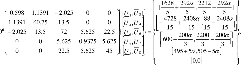
Therefore, the condensed equations (13) for uncertain distributed loads becomes
. 0,0 5 ,505 5 495 3 200 3 2200 , 3 200 600 15 2408 15 88 , 15 2408 15 4728 ] 5 292 5 2212 , 5 292 5 1628 [ = , , , , ] , [ 45 5.625 22.5 0 0 5.625 0.9375 5.625 0 0 22.5 5.625 72 13.5 2.025 0 0 13.5 60.75 1.1391 0 0 2.025 1.1391 0.598 10 8 8 7 7 6 6 4 4 3 3 6 U U U U U U U U U USolving the above fuzzy system of linear equations we get the lower and upper bounds of fuzzy static responses for triangular fuzzy loads and the obtained results are given in the table 1.
ISSN: 2231-5373 http://www.ijmttjournal.org Page 314
0 0.2 0.4 0.6 0.8 1
3 U
3 U
-0.4512e-3 -0.1931e-3
-0.4254e-3 -0.2189e-3
-0.3995e-3 -0.2447e-3
-0.3737e-3 -0.2705e-3
-0.3479e-3 -0.2963e-3
-0.3221e-3 -0.3221e-3
4 U
4 U
0.0567e-3 0.0620e-3
0.0573e-3 0.0614e-3
0.0578e-3 0.0609e-3
0.0583e-3 0.0604e-3
0.0588e-3 0.0599e-3
0.0594e-3 0.0594e-3
6 U
6 U
-0.2406e-3 -0.2621e-3
-0.2408e-3 -0.2600e-3
-0.2449e-3 -0.2578e-3
-0.2471e-3 -0.2557e-3
-0.2492e-3 -0.2535e-3
-0.2514e-3 -0.2514e-3
7 U
7 U
4.9996e-3 5.2999e-3
5.0296e-3 5.2699e-3
5.0596e-3 5.2398e-3
5.0897e-3 5.2098e-3
5.1197e-3 5.1798e-3
5.1497e-3 5.1497e-3
8 U
8 U
-0.5046e-3 -0.5314e-3
-0.5073e-3 -0.5288e-3
-0.5100e-3 -0.5261e-3
-0.5127e-3 -0.5234e-3
-0.5154e-3 -0.5207e-3
-0.5180e-3 -0.5180e-3
(a) (b)
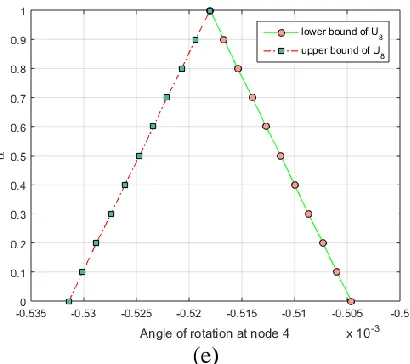
ISSN: 2231-5373 http://www.ijmttjournal.org Page 315 (e)
Figure 3. (a) and (d) represents the minimum and maximum bounds of transverse displacements at nodes 2 and 4 respectively. (b),(c) and (e) represents the minimum and maximum bounds of angle of rotations at nodes 2, 3 and 4 respectively of problem 1.
Example 2 :
Here we consider a two stepped indeterminant beam clamped at left end and whose right end is linear elastic spring supported with spring constant k. A rigid loading frame is placed at the middle of the beam which is subjected to a point load F0 as shown in figure 5. The beam is
discretized into two elements of equal length. On the first element an uniformly distributed load
0
q is acting. The material and geometric properties are considered crisp as
. 0.5 = , and / 10 = ; 4 = ; 10
50
= 6N m2 h m k 6Nm d m
EI
The elastic spring acting here as another finite element with element equation as
1 1
2 2
1 1
= (14)
1 1
e e
e e
u Q
k
u Q
ISSN: 2231-5373 http://www.ijmttjournal.org Page 316
Fig.4
The assembled equations are
1
1 1
2 2 1
2 2
1 2
3 3 1
2 2 2 1 2
4 4 2
3
2 3
5 3 1
2 2 2
6 4
3
7 2
12 6 12 6 0 0 0
6 4 6 2 0 0 0
12 6 18 3 6 3 0
2
=
6 2 3 6 3 0
0 0 6 3 6 3
0 0 3 3 2 0
0 0 0 0 0
U
h h q
U
h h h h q
U
h h h q q
EI
U
h h h h h h q q
h
U
h a h a q q
U
h h h h q
U
a a q
1 1 1 2
1 2
3 1
1 2
4 2
2 3
3 1
2 4 3 2
(15)
Q Q
Q Q
Q Q
Q Q
Q Q
3
w h e r e , = . 2
kh a
EI
With the given geometric and material properties the distributed load q0 and the concentrated load F0 are considered both as crisp and triangular fuzzy number to compute the static responses of the beam.
Case I(Crisp Load):
Let us consider the distributed load q0 and the point load F0 as crisp, where
. 5000 = ; / 10
= 3 0
0 Nm F N
q
The contribution of q0 to the element load vector is given by
] .3 4000 2000, , 3 4000 [2000,
= ] 6, , [6, 12 = ] , , , [
= 1 0
4 1 3 1 2 1 1
1 T T T
h h h q q
q q q
q
Since, there are no distributed loads on the other elements,the components of load vector
qi for(i=2,3) are zero. The global node 2 have a downward load of F0 =5000N. and bendingmoment of d.F0 =2500N.m. The specified global displacements, forces and balacced
equilibrium conditions are
0 = =
= 2 7
1 U U
U
= =5000 ., = . = 2500 . ., = 42 =0.
3 1 2 3 0
2 2 1 4 0
2 1 1
3 Q F N Q Q d F Nm Q Q Q
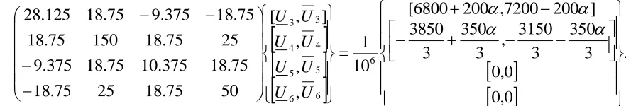
ISSN: 2231-5373 http://www.ijmttjournal.org Page 317 The condensed equations for the unknown global displacements are given by deleting the rows and columns corresponding to the specified global displacements. Thus, by deleting rows and columns 1,2 and 7, one may obtain the 44 matrix equations as
3 4 6 5 6 7000
28.125 18.75 9.375 18.75
3500
18.75 150 18.75 25 1
= 3 . (16)
9.375 18.75 10.375 18.75 10
0
18.75 25 18.75 50
0 U U U U
Solving the above systems we get the static responses as
. . 0.0568949 . 1.3744292 . 0.2768036 . 0.8536377 10 = 3 6 5 4 3 rad m rad m U U U U
Case II(Fuzzy Load):
Next, we consider the distributed load q0 and the concentrated load F0 as triangular
fuzzy number, where
. ,5100) (4900,5000 = ~ ; / ) 10 ,1.05 ,10 10 (0.95 = ~ 0 3 3 3
0 Nm F N
q
The corresponding interval forms in terms of cut of triangular fuzzy loads are given by
[0,1]. , where ], 100 ,5100 100 [4900 = ] , [ = ~ and ] 50 ,1050 50 [950 = ] , [ = ~ 0 0 0 0 0
0 q q F F F
q
The element load vector due to q~0 is
[6, ,6, ] =12 ~ = ] ~ , ~ , ~ , ~ [ =
~ 1 0
4 1 3 1 2 1 1
1 T T
h h h q q q q q q
3 200 3 4200 , 3 200 3 3800 100 ,2100 100 1900 3 200 3 3800 , 3 200 3 4200 ] 100 ,2100 100 [1900 = and the other two load vectors
q~ i (fori=2,3) are zero. The specified conditions of the internal forces for triangular fuzzy loads are] 100 ,5100 100 0.5[4900 = ~ . = ~ ~ ., ] 100 ,5100 100 [4900 = ~ = ~ ~ 0 2 2 1 4 0 2 1 1
3Q F N Q Q d F
Q
ISSN: 2231-5373 http://www.ijmttjournal.org Page 318
.
0,0 0,0
3 350 3
3150 , 3 350 3
3850
] 200 ,7200 200
[6800
10 1 =
, , ,
] , [
50 18.75
25 18.75
18.75 10.375
18.75 9.375
25 18.75
150 18.75
18.75 9.375
18.75 28.125
6
6 6
5 5
4 4
3 3
U U
U U
U U
U U
Solving the above systems we get the lower and upper bounds of fuzzy static responses and that are given in table 2.
Table 2: Lower and upper bounds of fuzzy static responses for triangular fuzzy load for example 2:
0 0.2 0.4 0.6 0.8 1
3 U
3 U
0.8435e-3 0.8638e-3
0.8455e-3 0.8618e-3
0.8475e-3 0.8597e-3
0.8496e-3 0.8577e-3
0.8516e-3 0.8557e-3
0.8536e-3 0.8536e-3
4 U
4 U
-0.2776e-3 -0.2760e-3
-0.2774e-3 -0.2762e-3
-0.2773e-3 -0.2763e-3
-0.2771e-3 -0.2765e-3
-0.2770e-3 -0.2766e-3
-0.2768e-3 -0.2768e-3
5 U
5 U
1.3838e-3 1.3651e-3
1.3819e-3 1.3669e-3
1.3800e-3 1.3688e-3
1.3782e-3 1.3707e-3
1.3763e-3 1.3726e-3
1.3744e-3 1.3744e-3
6 U
6 U
-0.0562e-3 -0.0576e-3
-0.0563e-3 -0.0575e-3
-0.0565e-3 -0.0573e-3
-0.0566e-3 -0.0572e-3
-0.0568e-3 -0.0570e-3
-0.0569e-3 -0.0569e-3
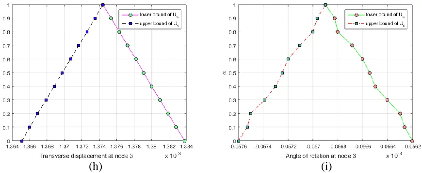
ISSN: 2231-5373 http://www.ijmttjournal.org Page 319 (h) (i)
Figure 5. (f) and (h) represents the minimum and maximum bounds of transverse displacements at nodes 2 and 3 respectively. (g) and (i) represents the minimum and maximum bounds of angle of rotations at nodes 2 and 3 respectively of the problem 2.
VI.CONCLUSIONS :
The static responses of some Euler Bernoulli’s beam problems using Fuzzy finite element method has been studied here. When the practical problems involve complecated shapes together with the loads involving uncertainties, the Fuzzy finite element method discussed here in a smooth way. In this paper we considered the loads as triangular fuzzy number only. This study can be extended to the other beam problems with loads as interval, trapezoidal and Type-2 fuzzy numbers. Instead of fuzzy loads one may consider the uncertainties in geometric and material properties. Matlab has been used to depict the results in terms of plots.
VII. ACKNOLEDGEMENTS:
We would like to thank RGNF (Rajib Gandhi National Fellowship), Govt. of India for providing fund to do this work.
VIII.REFERENCES :
[1]. O.C.Zienkiewicz, The Finite Element Method : Tata McGraw Hill Edition, 1979.
[2]. J.N.Reddy, An Introduction to the Finite Element Method : Tata McGraw Hill Edition, 2005. [3]. S.S.Bhavikati, Finite Element Analysis : New Age International Publisher, 2005.
[4]. I.Elishakoff, Probabilistic methods in the theory of Structures: New York ,Wiley, 1983.
[5]. A.Haldar and S.Mahadevan, Reliability Assessment Using Stochastic Finite Element Analysis. New York : John Wiley and Sons, 2000. [6]. L.Zadeh,Fuzzy Sets, Information and control, vol.8, pp. 338-353, 1965.
[7]. D.Dubois and H.Prade, “Operations on fuzzy numbers,” Inter. Journal of Systems Science, vol.9, pp.613-626, 1978. [8]. R.E.Moore, Methods and Applications of Interval Analysis, Philadelphia : SAIM Publication , 1979.
[9]. S.S.Rao and L.Berke, “Analysis of uncertain structural systems using interval analysis," AIAA Journal., vol. 35, pp. 727-735,1997. [10]. Z.Qui, X.Wang and J. Chen, “Exact bounds for the static response set of structures with uncertain-but-bounded parameters," Int. J. Sol. Struct., vol. 43, pp.6574-6593, 2006.
[11]. A.Chekri, G. Plessis, B.Lallemand, T.Tison, and P.level, “Fuzzy behavior of mechanical systems with uncertain boundary conditions," Comput. Methods Apll. Mech. Eng., vol.189, pp.863-873, 2000.
[12]. M.Hanss, Applied Fuzzy Arithmetic -An Introduction With Engineering Applications, Berlin : Springer-Verlag, ,2005.
[13]. S.S.Rao and J.P.Sawyer,“Fuzzy finite element approach for the analysis of imprecisely defined systems," AIAA J., vol.33, pp.2364-2370, 1995
[14]. U.O.Akpan, T.S.Koko, I.R.Orisamolu and B.K.Gallant, “Fuzzy finite element analysis of smart structures," Smart Mater. Struct., vol.10, pp.273-284,2001.
[15]. U.O.Akpan, T.S.Koko, I.R.Orisamolu, and B.K.Gallant, “Practical fuzzy finite element analysis of structures," Finite Element Analysis Des., vol.38, pp.93-111, 2001.
ISSN: 2231-5373 http://www.ijmttjournal.org Page 320
[17]. M.Hanss and K.Willner, “A fuzzy arithmetical approach to the solution of finite element problems with uncertain parameters," Mech.Res.Commun., vol.27, pp.257-272, 2000.
[18]. A.S.Balu and B.N.Rao,“Explicit fuzzy analysis of systems with imprecise properties," Int. J. Mech. Mater. Des., vol.7, pp.283-289,2011. [19]. A.S.Balu and B.N.Rao,“High dimensional model representation based formulation for fuzzy finite analysis of structures," Finite Elem. Anal. Des.,vol.50, pp.217-230,2012.
[20]. J.J.Buckley and Y.Qu, “Solving system of linear fuzzy equations," Fuzzy Sets and Systems, vol.43, pp.33-43, 1991. [21]. D. Dubois and H. Prade, Fuzzy Sets and systems: Theory and Applications, New York : Academic Press 1980. [22]. M.Friedman, M.Ming and A.Kandel,“Fuzzy linear systems," Fuzzy Sets Syst., vol.96, pp.201-209, 1998.
[23]. X.Wang, Z.Zong and M.Ha, “Iteration algorithms for solving a system of fuzzy linear equations," Fuzzy Sets and Systems, vol.119, pp.121-128, 2001.
[24]. A.Kauffman, M.M.Gupta, Introduction to Fuzzy Arithmetic:Theory and Applications, New York : Van Nostrand Reinhold, 1991. [25]. D. Dubois and H. Prade, “The mean value of a fuzzy number," Fuzzy sets and Systems, vol.24, pp.279-300, 1987.
[26]. O.Kaleva, “Fuzzy differential equations," Fuzzy Sets and Systems, vol.24, pp.301-317, 1987.