Quantifying the trends expected in developing ecosystems
Michael T. Mageau *, Robert Costanza, Robert E. Ulanowicz
Uni6ersity of Maryland Institute for Ecological Economics,Center for En6ironmental and Estuarine Studies,Uni6ersity of Maryland,
PO Box38,Solomons,MD20688,USA
Received 21 November 1997; accepted 16 April 1998
Abstract
In this paper we describe an assessment of ecosystem health that is both comprehensive in that it is based on a series of common trends associated with the process of ecological succession, and operational in that the indices capable of quantifying these trends can be easily calculated given appropriate simulation model output or estimates of material exchange. We developed a simulation model which generated output characteristic of an ecosystem advancing through the various stages of succession to test the ability of a suite of systems-level information indices to quantify these trends. Our regression analyses suggest that these indices may be able to capture the trends associated with ecological succession, hence the reversal of many of these trends characteristic of ecosystem response to anthropogenic stress. We further argue that indice performance could be enhanced with the use of more dynamic modelling techniques. In addition, we introduce a methodology for the valuation of non-marketed ecosystem components which could be easily included with our assessment of ecosystem health. We conclude that this measure of ecosystem health in combination with the valuation technique may provide an informative compliment to many past and future regional modelling projects aimed at better understanding and managing the impacts of anthropo-genic stress on our regional ecosystems. © 1998 Elsevier Science B.V. All rights reserved.
Keywords: Ascendancy; Ecosystem health; Ecosystem management; Ecological succession; Network analysis; Sustain-ability
1. Introduction
We need to arrive at a healthy balance between our stocks of human-made (HMC) and natural
capital (NC) if we are to continue to survive on this planet. In the past, we have been largely unable to quantify the effects of anthropogenic stress on our natural ecosystems with the degree of certainty required to influence policy decisions. Popper (1990) argues that the natural world is causally open at all scales of observation includ-ing those occupied by ecosystems, and suggests * Corresponding author. Present address: 5815 Glenwood
Street, Duluth, MN 55804, USA. Tel.: +1 218 5255311; fax: +1 410 3267354; e-mail: [email protected]
our inability to predict ecosystem behaviour (Abrams, 1994) is due not to lack of information regarding system dynamics, but to the fact that these systems are intrinsically indeterminate. Therefore, rather than continue to pursue the unattainable goal of predicting ecosystem be-haviour, we must begin to use our best current information to reach consensus on predictions of what factors would likely lead to the sustainability of ecosystem structure and function, and develop policy in a flexible, adaptive framework capable of incorporating rather than obviating this uncer-tainty (Costanza and Ruth, 1998). Crucial to this task is the development of a systems-level measure of ecosystem health which is comprehensive, oper-ational and capable of encompasing the uncer-tainty associated with ecosystem dynamics.
1.1. Definitions and measures of ecosystem health
Many researchers have attempted to define and develop operational and meaningful definitions and indicators of ecosystem health. Leopold (1941) contributed to the practice of ‘land health’ by identifying indicators of ‘land sickness’. Rap-port et al. (1985) expanded on Leopold’s original indicators arriving at what he called ecosystem distress syndrome (EDS). Costanza (1992) sum-marized the wide variety of proposed concept definitions of ecosystem health based on EDS: Health as homeostasis; as absence of disease; as diversity or complexity; as stability or resilience; as vigor or scope for growth; and as balance between system components. Karr et al. (1986) stated that a biological system can be considered healthy when its inherent potential is realized, its condition is stable, its capacity for self repair when perturbed is preserved, and minimal exter-nal support for management is needed. Kerr and Dickey (1984) suggested evaluating ecosystem health using the size distribution of biota. Schaef-fer and Cox (1992) stated that health is achieved when functional ecosystem thresholds are not ex-ceeded. Schindler (1990) provided a detailed ac-count of whole lake acidification experimentation demonstrating a sequence of abnormal signs of ecosystem structure and function. Smol (1992) defined a healthy ecosystem as one that existed
prior to human cultural impact. Odum (1985) and Ulanowicz (1986) suggested that stressed ecosys-tems are characterized by an inhibition or even reversal of the trends associated with ecosystem development. Costanza (1992) suggested that an ecosystem is healthy if it is stable and sustainable that is if it is active, maintains its organization and autonomy over time and is resilient to stress. Finally, there is a related body of literature that uses the term ‘integrity’ in place of ‘health’ when referring to ecosystem transformations under stress, and they generally consider a healthy ecosystem to be pristine (Karr, 1993; Kay, 1993; Woodley et al., 1993; Westra, 1994).
metabolism or production. Organization is a mea-sure of the number and diversity of interactions between the components of a system, and re-silience refers to the ability of a system to main-tain its structure and function in the presence of stress (Mageau et al., 1995). Costanza and Patten (1995) describe the debate surrounding the defini-tion of sustainability, and suggest that much of the discussion is misdirected because sustainability is not a definitional concept, but more one of prediction. For example, you cannot demonstrate the sustainability of any ecosystem until after the fact, much like the fitness of an organism. When applied to complex systems such as ecosystems, predictions regarding sustainable configurations are typically highly suspect, and as such should be subjected to elaboration, discussion and debate. Maintaining the sustainability of a system’s vigor, organization and resilience embodies all the defin-itions of ecosystem health discussed above.
1.2. Trends associated with ecosystem response to stress
Fortunately for our purposes, the literature contains a rich history documenting robust trends or patterns associated with the response of a wide variety of ecosystems to many different perturba-tions. These trends are specific enough to be quantified with a unique suite of indices, and yet comprehensive enough to serve as meaningful, systems-level indicators of ecosystem response to anthropogenic stress.
Woodwell (1967) described various changes in ecosystem structure and function typically associ-ated with the natural process of ecological succes-sion: (1) diversity tends to increase as new niches are occupied; (2) competition increases efficiency and reduces redundancy within a given niche while decreasing the level of competition between niches; (3) nutrient inventories, storage and
cling increase; (4) the structural and functional stability of the ecosystem increases, and the ratios of production per unit biomass and respiration tend to decline. If, during this process of succes-sional development, one or more factors essential to the system became exhausted or limited, the process of succession is halted or slowed, respec-tively. Woodwell (1967) further reasoned that if the system was exposed to an extreme natural or anthropogenic stress, the successional develop-ment would not only be halted but reversed. Therefore, the opposite of the trends discussed above would indicate an ecosystem that is stressed. Woodwell (1967) tested these hypotheses by irradiating a section of climax oak/pine forest, and found the pattern from the zone receiving the highest levels of radiation to the lowest was the exact opposite of the pattern of natural succession.
Woodwell (1970) further discussed the implica-tions of his findings in the ‘irradiated forest.’ He was struck by the fact that changes in vegetation patterns along the gradient of radiation exposure were similar to those found along natural gradi-ents of increasing environmental stress such as those associated with increasing elevation along exposed mountain slopes, salt spray and water stress. He also found that the species surviving intense radiation were very similar to those found in typically stressed areas such as roadside ditches, gravel banks and places with unstable soils. In addition, the changes in his climax forest system paralleled those found in association with the oxides of sulphur radiating from Sudbury’s smelters (Gorham and Gordon, 1960) and the replacement of Vietnam’s extremely diverse forest canopies with bamboo in the wake of massive herbicide applications (Tschirley, 1969).
Odum (1985) developed a more complete list of certain well defined development trends to be expected in stressed ecosystems, and provided a history of theoretical and empirical evidence doc-umenting their occurrence. Odum (1985) argued that increasing community respiration, unbal-ancedP/Rratios, increasingP/BandR/Bratios, increasing dependence on external energy, and increased export of unused primary production are energetic trends to be expected in stressed
ecosystems. He also provided evidence of in-creased nutrient turnover, horizontal transport and loss from stressed ecosystems coupled with decreasing internal nutrient cycling. In addition, Odum (1985) highlighted several changes in com-munity structure and function. The proportion of R-strategists tends to increase while the size and life-span of organisms tends to decrease. Food chains shorten as the result of reduced energy flow to higher trophic levels, and biodiversity tends to decline along with an increase in the redundancy of parallel pathways of material exchange. Fi-nally, Odum (1985) suggested evidence of these trends may serve as an excellent ecosystem-level indicator of stress.
Schindler (1990) tested Odum’s hypotheses re-garding the trends expected in stressed ecosystems by analyzing the effects of nutrient enrichment and acidification on whole-lake ecosystems. Schindler’s analysis supported Odum’s hypotheses to a large extent. For example, the acidified lakes were characterized by: increased periphyton com-munity respiration, P/R ratios, nutrient export, R-strategists among zooplankton, and decreased utilization of allochthonous inputs, vertical cy-cling of nutrients, life-spans of fishes, benthic crustaceans, sizes of zooplankton and chirono-mids, length of food chain, species diversity and efficiency of resource use, all of which support Odum’s hypotheses. Schindler also found no evi-dence of increasing P/B and R/B ratios, no change in exported primary production, a de-crease in the horizontal transport of nutrients, a decrease in R-strategists among the fish, and an increase in the average size of phytoplankton all of which apparently contradict Odum’s hypothe-ses, but the majority of these exceptions were explained within the confines of the paradigm. In the eutrophied lakes Schindler (1990) again found general support for Odum’s hypotheses, despite a few apparent, often explainable, exceptions.
and ecosystem stability. Elton (1958) suggested decreased diversity would lead to decreased ecosystem stability. McNaughton (1977) pre-sented data on plant productivity in the Serengeti supporting Elton (1958) and Vitousek and Hooper (1993) found the rates of many ecosystem processes were increasing but saturating functions of species diversity. On the other side of the debate, May (1973) using a simple model of multi-species competition showed population dynamics were progressively less stable as the number of competing species increased. Others (DeAngelis, 1975; Gilpin, 1975; Pimm, 1979) reached similar conclusions resulting in a consensus lasting two decades that decreased population stability would lead to decreased ecosystem stability.
Tilman et al. (1996) provided evidence from 12 years of experimentation with 207 grassland plots exposed to the stress of extreme drought that both sides of the debate were correct, and only the assumption that less species stability would lead to less ecosystem stability was in error. Tilman et al. (1996) found that year to year variability in total community biomass was lower in high diver-sity plots, and the change in community biomass resulting from the stress of drought was nega-tively correlated with diversity. Finally, in addi-tion to resistance, they found the plots with a higher species diversity recovered more quickly as well (resilience). He also found year to year vari-ability in species abundance was not stabilized by biodiversity suggesting that biodiversity stabilizes community and ecosystem processes, but not pop-ulation processes. He concluded the difference between species and community biomass resulted from inter-specific competition when stress nega-tively impacts some species others are allowed to proliferate maintaining ecosystem function while increasing variability in species abundance.
In addition, the literature documents evidence of a positive relationship between biodiversity and productivity. Naeem (1994) looked at the rivet (Ehrlich and Ehrlich, 1981) versus the redundancy (Walker, 1992) hypotheses which mark the ex-tremes along a continuum of belief regarding the contribution of individual species to ecosystem function. They worked with three different levels of biodiversity and found system production was
highest in the most diverse system, and that pro-duction levels varied less than in the less diverse systems. Tilman and Downing (1994) found the stress of drought resulted in less production de-cline in more diverse plots, and that the more diverse stands recovered quicker. Tilman et al. (1996) presented evidence supporting both the diversity-productivity and the diversity-sustain-ability hypotheses. They found more diverse plots were able to achieve higher productivity, and argued this was because more variety in the strat-egy of nutrient use by more diverse plant commu-nities allows for more efficient use of nutrients leading to more production. They also reported evidence supporting the diversity-sustainability hypothesis by finding less nutrient leaching in the more diverse plots, and arguing that biodiversity tightens nutrient cycles leading to more sustain-able soil fertility.
Finally, there are more specific aspects of diver-sity that contribute unequally to ecosystem func-tion. Walker (1995) argues that species diversity and functional diversity are important, but the diversity of species within each functional guild is most crucial to maintaining ecosystem function. Therefore, he suggests that when protecting biodi-versity one should ensure functional dibiodi-versity by protecting those species associated with functional guilds containing relatively few species. As Schin-dler (1990) and Tilman et al. (1996) noticed ecosystem function can be maintained despite loss of species diversity until the final species repre-senting functional guilds begin to disappear. Of-ten it is not enough to maintain high species diversity, but we must be careful to ensure high diversity within each particular guild to maintain overall system function in the face of external stress.
1.3. Quantifying the trends expected in stressed ecosystems
in-formation (I); (3) system uncertainty (H); (4) system ascendancy (A); (5) development capacity (C) and (6) system overhead (L). These indices stem from a unique and controversial background involving causality in natural phenomenon (Ulanowicz, 1997). For example, Popper (1990) argued that we live in a world of ‘propensities’ which characterize the probability of the occur-rence of any event given the situation in which the event occurred. According to Popper, the vast majority of events can be characterized by condi-tional probabilities with intermediate values (be-tween 0 and 1). It is extremely rare to find an event characterized by a conditional probability of 1 (pure deterministic force) or of 0 (purely random chance of occurring). Ulanowicz (1997) argues the universe is causally open at all scales including ecosystems, and although many events may tend to happen with high probabilities there is no fundamental determinism underlying ecosys-tem behaviour. He stresses that any setback in scientific progress due to acknowledging chance at the ecosystem scale could be more than offset by new discoveries emanating from a new perspec-tive, and offers quantum physics as an example. In short, chance is part of any ecosystem transac-tion, and the conditional probability of any event in an ecosystem can be calculated as well as the changes in these probability assignments concur-rent with changes in ecosystem structure and function, and it is these changes in probability assignments that drive the behaviour of Ulanow-icz’s (1986) indices.
Ulanowicz (1986) identifies mutualism or auto-catalysis between system components, connected by cyclic flow, as the underlying phenomenon influencing the changes in ecosystem structure and function measured by the indices. In autocatalysis an increase in the activity of any component increases the activity of all other members in the cycle and ultimately itself, resulting in configura-tions that are growth enhancing via positive feed-back. These autocatalytic configurations also exert selection pressure on their members. If a more efficient species enters the cycle, its influence on the cycle will be positively reinforced, or if the species is less efficient, negative reinforcement will decrease its role. In addition, as the autocatalytic
cycle increases it’s activity it absorbs resources from its surroundings. Therefore, as ecosystems undergo the process of succession in the absence of stress, autocatalysis increases the amount of material being transported throughout the system and the efficiency by which its members exchange material and energy. Finally, different members may come and go, but the fundamental structure of the autocatalytic cycle remains making the loop independent of its constituents. Therefore, Ulanowicz argues that autocatalysis streamlines the topology of interconnections in a manner that favours those transfers that more effectively en-gage in autocatalysis at the expense of those that do not, resulting in networks that tend to become dominated by a few intense interconnecting flows. TST is the most straight forward of the six indices. It is simply a measure of the sum total of all the inputs, outputs and materials being trans-ferred between components within the system at any given point in time. AMI is a measure of the information we have regarding the network of material exchange within the system. If material from any particular component in the system had an equal chance of flowing to any of the potential recipients then we would have no information regarding the flow network, however, if all mate-rial from a particular component was transferred to only one of the potential recipients, we would have complete information regarding the flow structure. These extreme information values never occur in ecosystems, but, Ulanowicz (1986) hy-pothesizes that AMI increases with ecosystem suc-cession as autocatalytic competition streamlines the network of material exchange.Ais simply the product of AMI and TST. Ulanowicz (1980) hy-pothesized that A increases with successional ecosystem development as autocatalysis increases both TST and AMI.
succes-sion. TST is limited by the amount of input in combination with the second law of thermody-namics. H increases as a given amount of TST is partitioned among a greater number of exchange pathways associated with an increase in diversity. But, as the diversity increases, the smallest units are more likely to succumb to chance perturba-tion, hence the flow diversity H cannot increase forever. Therefore, C is limited by the limits on TST and H.
Overhead (L) is the difference between capacity and ascendancy (C−A). Ulanowicz (1980) hy-pothesized that as ecosystems undergo the process of developmental succession, A approaches C at the expense of L. At first, both A and C will increase with succession, but ultimately Cwill be limited. However, A can continue to increase at the expense ofL. A certain level ofLis crucial to the maintenance of ecosystem structure and func-tion, hence there are limits to this trade-off of A for L. Ulanowicz (1997) partitions L into four categories: inputs, exports, dissipations and path-way redundancy, and describes the factors which constrain their magnitude.
The contribution of input overhead to total overhead decreases as a given magnitude of input is partitioned into ever fewer recipient categories. A trade-off develops between the benefits of con-centrating input in the most efficient input path-ways, and the vulnerability of relying extensively on too few input pathways. A decrease in the fraction of input to TST also leads to a decrease in the contribution of input overhead to total overhead. Dissipation overhead decreases with the fraction of respiration to TST, and as the distri-bution of respiration among system components becomes more equitable. Overhead on useable exports decreases with the utilized proportion of these exports, and the contribution they make to further increases in TST. Finally, overhead result-ing from pathway redundancy decreases as the network of material exchanges becomes stream-lined by the process of autocatalysis. A trade-off develops between the increasing efficiency result-ing from a network of exchanges dominated by only the most efficient transfers, and the vulnera-bility resulting from the rigidity of such a flow configuration.
In summary, Ulanowicz (1986) offers the fol-lowing description of ecological succession rela-tive to his indices. In the early stages of ecological succession C, A and L increase due to the dra-matic increase in TST associated with the pulse of growth provided by abundant resources. In the later stages of succession, resource limitation ini-tiates the replacement ofr-selected species by the more specialized and efficient k-selected species. This shift in species composition leads to higher levels of species and functional diversity increas-ing TST by allowincreas-ing the system to better utilize limiting resources, and more efficiently transfer biomass to higher trophic levels. In addition, this shift in species composition triggers an increase in H as new flow pathways continue to evolve while new niches are exploited. AMI also increases as the flow network is streamlined to favour only the most efficient material transfers within each niche or functional guild. This competition within each niche leads to a decrease in overhead as redun-dant flow pathways are eliminated and mortality, export and respiration rates decrease. At some point the species occupying the most fragile of niches are eliminated by chance perturbation de-pending on the frequency and severity of natural or anthropogenic stress. This phenomenon pro-vides an upper bound to the potential for in-creases in H, and the laws of thermodynamics provide an upper bound on TST resulting in an upper bound onC. At these later stages of ecolog-ical succession TST,H andCessentially level off, but AMI can continue to increase relative to H, hence, Arelative to Cat the expense ofL.Awill continue to increase at the expense of L with C remaining essentially constant until the network of exchanges becomes to brittle or vulnerable to any change in external conditions. Each system develops an optimal balance between A and L depending on the variability of its external envi-ronment. Therefore, the indices taken in combina-tion may be capable of quantifying the trends associated with the process of ecological succes-sion, and the reversal of these trends apparent in ecosystems subjected to anthropogenic stress.
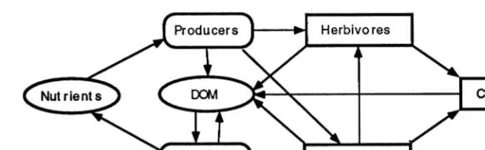
Fig. 2. A general diagram depicting the interactions between the major trophic levels in the general ecosystem model. ecosystem model capable of depicting a range of
behaviour typical of various stages of ecological succession. The resulting correlations support our hypotheses regarding indice response to succes-sional trends suggesting the indices may be used to measure the response of any particular ecosys-tem to stress provided it is characterized by an appropriate, well-calibrated simulation model, or data directly characterizing material exchanges between system components.
2. Materials and methods
2.1. Model de6elopment
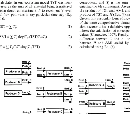
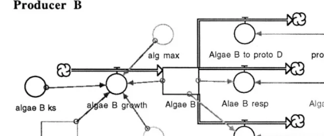
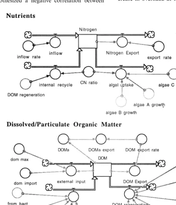
We constructed a simple pelagic ecosystem model in STELLA to test the ability of Ulanowicz (1986) system-level, information indices to quan-tify the trends described above. There were five major living components in the model represent-ing four trophic levels, and two nonlivrepresent-ing storages of nutrients and organic matter (DOM) (Fig. 2). Each trophic level contained several different spe-cies with differing degrees of functional specializa-tion (Fig. 3). The ‘A’ species in each trophic level represented generalists (also the ‘B’ species in the protozoan and carnivore trophic levels), and the ‘B, C, D and E’ species in each trophic level repre-sented specialists. In addition, the various model coefficients were adjusted to assign the generalist species growth kinetics typical of R-strategists (high growth rates, high nutrient Ks values, high respiration rates etc…), and the same was done with the specialists to make their growth kinetics
typical of k-selected species (low growth rates, low nutrientKsvalues etc…). Therefore, when the system was dominated by the ‘A’ species it exhib-ited behaviour typical of an early succession ecosystem, and when the system was dominated by the ‘B/C/D/E’ species it exhibited behaviour typical of a late successional ecosystem.
The relative dominance of any particular pro-ducer or bacterial species depended largely on their growth rates, respiration rates and their abilities to utilize available supplies of nutrient and DOM, respectively (Fig. 4). The relative dom-inance of species in higher trophic levels depended largely on their feeding efficiencies, respiration rates, mortality rates and the species distribution at the producer and bacterial trophic levels (Fig. 4). However, there were also important ‘top down’ feedbacks which depended on the feeding rates and efficiencies of the species present in the higher trophic levels. The net result of this dy-namic tension between ‘bottom up’ and ‘top down’ feedback mechanisms was model output characteristic of an ecosystem advancing through the various stages of ecological succession.
2.2. Indice calculation
We calculated Ulanowicz (1986) system level information indices within the STELLA model, so we could track these values over the course of any simulation. Ulanowicz (1986) describes the calcu-lation of the network analysis based, systems level information indices in detail, so we provide only a brief summary in this paper. Of the three network measures TST was the most straight forward to calculate. In our ecosystem model TST was mea-sured as the sum of all material being transferred from donor compartment ‘i’ to receipient ‘j’ over all flow pathways in any particular time step (Eq. (1)).
TST=%Tij (1)
AMI=%Tijlog(TijTST/TjTi) (2)
H=%Tij/TSTlog(Tij/TST) (3)
A=TSTAMI (4)
C=TSTH (5)
L=C−A or =TST(H−AMI) (6)
AMI andHrepresented the sum of each unique individual compartment’s information and uncer-tainty values, and were calculated within the sim-ulation model using Eqs. (2) and (3), respectively. WhereTiis the sum of all material leaving theith
component, and Tj is the sum of all material
entering the jth component. Ascendancy is simply the product of TST and AMI, and capacity is the product of TST andH(Eqs. (4) and (5)). We have chosen this particular form of ascendancy in place of the more comprehensive biomass-inclusive ver-sion because it has a definitive upper bound which allows the calculation of corresponding overhead values (Ulanowicz, 1997). Finally, overhead is the difference between C and A, or the difference between H and AMI scaled by TST, and was calculated using Eq. (6).
Fig. 4. The conceptual diagram and growth equation for a primary producer which is representative of the bacterial species as well, and a protozoan which is representative of all species in higher trophic levels.
2.3. Hypotheses and regression analyses
We formulated several hypotheses regarding the response of the indices to the trends discussed above, and tested them by regressing the ratio of the biomass representing the sum of species ‘A’ biomasses (and the ‘B’ species in the protozoan and carnivore trophic levels) to the total system biomass with TST, AMI, H, A, C and L. Our hypotheses were divided into those regarding
ascendancy and species ‘A’ resulting from a de-crease in TST and a relative inde-crease in overhead. Finally, from a community structure perspective, dominance by the ‘A’ species should have lead to a relative increase in r-selected species dynamics, and a decrease in the diversity of functional guilds participating in the system. We hypothesized that these trends would lead to a decrease in capacity, ascendancy and overhead, and to a relative in-crease in overhead at the expense of ascendancy. and a negative correlation between ascendancy and
dominance by species ‘A’. From a nutrient per-spective, the ‘A’ species were characterized by low Ks values, and were ingested less efficiently by higher trophic levels. In addition, a percentage of each were lost from the system. These characteris-tics should have lead to a decrease in the efficiency by which nutrients are cycled within the system, and a loss of nutrients from the system. Therefore, we hypothesized a negative correlation between
Overall, dominance by members of the ‘A’ spe-cies should have produced behaviour characteris-tic of early successional ecosystems which should have lead to increases in overhead at the expense of ascendancy for any given capacity and TST. Whereas, an increase in dominance by members of the B, C, D, and E species should have pro-duced behavior characteristic of late successional ecosystems which should have lead to relative increases in ascendancy at the expense of over-head for any given capacity and TST. In addition, dominance by the more efficient species B, C, D and E should lead to an overall increase in TST, AMI andH, and drive corresponding increases in ascendancy, capacity and perhaps overhead de-pending on the relative influence of TST.
3. Results
3.1. Component biomass 6alues
Fig. 6 depicts the carbon biomass of each sys-tem component over the course of the entire simulated successional event. Supplies of available nutrient and DOM declined to limiting levels by the midpoint of the simulation, and remained at those levels for the duration. The primary pro-ducer and decomposer components displayed sim-ilar behaviour. The total biomass of each component category increased throughout the en-tire simulation while species B and C essentially replaced species ‘A’ by the midpoint of the simu-lation. The protozoans and herbivores exhibited the same basic pattern including an increase in total biomass throughout the entire simulation along with a replacement of the generalist species by the specialists around the midpoint of the simulation. Finally, carnivore biomass also in-creased throughout the entire simulation, how-ever, the C, D and E species were unable to completely replace the A and B species as they did in the other trophic levels.
3.2. Network information indices
Fig. 7 depicts the response of the systems-level, network, information indices to the component
biomass results described above. Capacity (C) and its two components overhead (L) and ascen-dancy (A) increased throughout the first half of the simulation, and then levelled off in the second half. Average mutual information (AMI) also in-creased in the first half of the simulation and then levelled off in the second. System uncertainty (H) increased rapidly at the start of the simulation, double-peaked and then declined by the midpoint remaining constant for the latter half. Finally, total systems throughput (TST) increased throughout the entire simulation, but at a slower rate in the latter half.
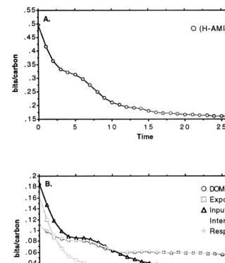
Fig. 8 illustrates the response of overhead and its five components per unit TST to the simulated results described above. This total weighted over-head index declined throughout the entire simula-tion, but at a more rapid rate in the first half. The five components of overhead also declined throughout the entire simulation, but at differing rates. The weighted measures of export and input overhead declined at the fastest rate, DOM and respiration overhead components declined at an intermediate rate, and the overhead attributed to internal transfers declined at the slowest rate.
3.3. Regressions:biomass ratios 6ersus indices
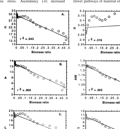
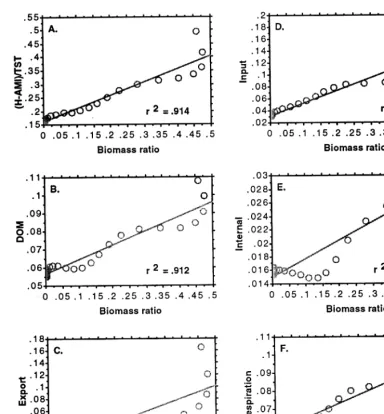
Fig. 9 illustrates the relationship between the various network indices and the ratio ofr-selected species biomass to total system biomass (BR). There was a strong negative correlation between C, A, AMI and TST (R2=0.94, 0.97, 0.96, 0.96, respectively) and the BR. L was also negatively correlated with the BR, but the correlation was not as strong (R2=0.88). However, the overall L/TST measure was positively correlated with the BR (R2=0.91). Finally, there was no correlation between the BR and H (R2=0.02).
4. Discussion
4.1. Simulated successional changes in species composition
eco-Fig. 6. The biomass value in carbon of each of the main system components throughout the entire simulated ecological succession event. Each graph depicts all the species within a given trophic level. (A) Nutrients and DOM; (B) primary producers; (C) bacteria; (D) protozoans; (E) herbivores; (F) carnivores.
logical succession discussed above (Woodwell, 1967; Odum, 1985; Rapport et al., 1985; Tilman et al., 1996). In our model the relative supply of Nutrient and DOM influenced the species com-position and relative biomass of the primary producer and decomposer trophic levels respec-tively (Fig. 6A,B,C). The r-selected species in
turn influenced the species composition and relative biomass of species representing the higher trophic levels. In general, as the levels of DOM and nutrient
declined throughout our simulated version of eco-logical succession the k-selected species replaced the r-selected ones at the lowest trophic levels
Fig. 8. The value of total system overhead (A) and its five components (B) divided by TST over the entire simulated ecological succession event. Units are in bits/carbon.
leading to similar species compositional shifts at successively higher trophic levels (Fig. 6D, E, F).
Due to the differing characteristics of our sim-ulatedr andk-selected species the above compo-sitional shifts led to the following changes in system characteristics: (1) higher biomass values within each trophic level as species with more efficient growth kinetics better incorporated lim-iting resources, and more efficiently transferred their biomass to successively higher trophic lev-els; (2) increased TST as higher biomass values led to more material transfer between compo-nents; (3) a more streamlined flow network as
4.2. Indice response to simulated successional trends
In general the system-level, information indices responded to our simulated ecological succession event as hypothesized indicating that they may serve as a useful measure of the trends associated with ecological succession, hence, the arrestment or reversal of these trends associated with anth-ropogenic stress. Ascendancy (A) increased
throughout the simulation due to increases in its two components AMI and TST (Fig. 7A, B, D). The rate of increase in A, AMI and TST was greatest in the first half of the simulation corre-sponding to the gradual replacement of r-selected species by the more efficient and specialized k -se-lected species within each trophic level. The greater efficiency of the k-selected species led to higher levels of TST, and their specialization (fewer pathways of material exchange per species)
led to higher values of AMI. After the midpoint of the simulation the rate of increase in AMI was near zero, whereas TST and A continued to in-crease, but at a much slower rate. Steady co-dom-inance by the limited number ofk-selected species in the second half of the simulation likely con-strained any further rise in AMI, and the gradual increase in TST as the result of slowly increasing biomass fueled the slight rise in A.
Capacity (C) increased throughout the simula-tion in a manner similar to that of TST. However, at the midpoint of the simulation there was a slight decline in capacity which corresponded with the noticeable decline in uncertainty (H) following its double peak (Fig. 7A, C, D). Uncertainty is a measure of the diversity of material exchange pathways, and increases as a given amount of TST is more equally partitioned into ever more pathways (Ulanowicz, 1986). The double peaks in uncertainty corresponded to the period in the simulation when all species existed as the special-ists were slowly replacing the generalspecial-ists. It was at this unique point in the simulation when the number of pathways of material exchange per unit system throughput was at its peak. H then levelled off after a steep decline corresponding to the point when the generalist k-selected species completely out competed their r-selected counter-parts and dominated for the remainder of the simulation. Therefore, the behaviour of capacity was largely the result of TST, but the slight decline at the midpoint of the simulation, and the decreased slope in the second half of the simula-tion was attributed to declines inH.
Overhead (L) also increased throughout the simulation in a manner similar to TST. However, L showed a slight peak at the midpoint of the simulation followed by a gradual decline in the third quarter, and then a gradual increase in the fourth.Lis measured as the difference betweenC and A, or as TST(H−AMI) (Ulanowicz, 1986). Because AMI was nearly constant for the entire second half of the simulation the behaviour of L was largely determined by the rate of increase in TST and decline in H. In the third quarter of the simulation the rapid decline in H overcame the slight increase in TST resulting in the slight de-cline inL. In the fourth quarter of the simulation
H levelled off and the slight increase in L was attributable to the slight increase in TST.
This behaviour in L was inconsistent with our hypotheses. According to theory (Ulanowicz, 1986) overhead should decrease with ecological succession as A approaches C, or AMI ap-proaches H. These phenomena occur as the more efficient specialists tend to dominate the food web resulting in a greater diversity of flow pathways, but fewer connections per node, less mortality, less respiration and export per unit biomass, and inputs which are partitioned into fewer compo-nents. L increased throughout the simulation be-cause of the dominant influence of TST. However, L/TST declined throughout the simulation in a manner more consistent with our hypotheses (Fig. 8A). In addition, each of the five components of overhead also declined throughout the simulation when corrected for the dominant influence of TST (Fig. 8B). Further evidence supporting our hy-potheses comes from the fact that AMI ap-proachesHin the second half of the simulation as AMI remains constant while H declines, and this leads to a slight convergence in the A and L curves as A makes up a larger proportion of C (Fig. 7A, B, C).
Fig. 10. (A) A phase-plane plot of the relationship between the value of total system overhead per unit TST and the biomass ratio; (B – F) the relationship between each of the five components of overhead per unit TST and the biomass ratio.
the BR and the overhead values per unit TST (Fig. 10A, B).
4.3. Limitations of simulation modelling
Overall, the behaviour of the suite of network indices in relation to our simulated ecological succession event was largely consistent with Ulanowicz (1986) theory of indice response to
In the second half of our ecological succession event TST,C, and Acontinue to increase slightly while AMI,H and L essentially level off. The continued increase in TST,CandAare consistent with our hypotheses, however we also suspected AMI would continue to increase while H re-mained fairly constant and L declined. In hind-sight these apparent contradictions can be attributed to limitations imposed by our simula-tion model that would likely be absent in natural systems. For example, in our model the maximum number of species in each trophic level was either three, four or five. This resulted in a cap on the value ofH, and the peaks in Hcorresponding to the points in the simulation when all species were co-dominant. Beyond this point as thek-selected species attained clear dominance biodiversity and H actually declined from their co-dominance peaks. In a natural system as diversity increases with succession H would likely continue to in-crease well beyond the levels representing the relatively early successional co-dominance of r and k-selected species. This suggests that deter-mining the appropriate levels of aggregation may be crucial to the success of using simulation mod-els in combination with the network indices to measure the health of any given ecosystem.
Another problem with our simulated succession event was that TST tended to dominate the more interesting contributions of AMI and H through-out the entire simulation. In the later stages of succession changes in AMI and H should domi-nate the relatively small changes in TST. The problem is that ecosystem simulation models are typically rigid in structure, and offer only a me-chanical description of ecosystem dynamics. Once the original framework of a model is set, the values representing the component biomasses and their interconnecting flows can vary dramatically, but new components or pathways of medium exchange between them (changes in network to-pology) often cannot arise, nor can previous ones disappear.
Ulanowicz (1986) indices are sensitive to both changes in the relative magnitude of medium transferred within a static network topology, and changes in the actual topology itself. In our simu-lation model, the network topology was fixed, so
our indices were only responding to the first of these two factors, and TST tended to dominate the more subtle effects of AMI andH. In natural systems, of course, the topology of food webs are not fixed. A simulation model capable of captur-ing each of these factors would lead to far more variability in the measures of AMI and H, hence A,C and L. Jorgensen (1986, 1988a,b, 1992) de-scribes a new generation of structurally dynamic simulation models based on goal functions which evaluate the unique parameter set that optimizes the function at each particular time step, and which may be capable of depicting the interesting changes in network topology often missed by more traditional modelling approaches. It is cru-cial to develop these more dynamic simulation models capable of simulating changes in network topology if Ulanowicz (1986) indices are to be used to measure the hindrance or reversal of the trends associated with ecological succession.
Christensen (1995) used Odum (1969) list of successional attributes to develop and index of ecosystem maturity, and examined the correlation between his maturity index and many of Ulanow-icz (1986) indices using 41 steady-state models of aquatic ecosystems. Christensen found that over-head was positively correlated with his index of system maturity. This is in agreement with our findings discussed above, although counter to Ulanowicz (1980) hypothesis. As described above, we suggest that the dominating effects of increas-ing TST along with ecological succession or matu-rity relative to the more subtle effects of AMI and H typical of topologically rigid simulation model output may explain this apparent positive correla-tion. In fact, Costanza suggests replacing TST with net system throughput (NST) which would simultaneously avoid the problems associated with the dominant effects of TST over H and AMI, and make the analysis independent of scale or the level of system aggregation.
some point in the later stages of ecological succes-sion the value of H will no longer increase as chance perturbations effectively trim further in-creases in diversity. However, AMI can continue to increase despite the relatively constant value of Has a greater proportion of material flows along the most efficient transfer pathways. Prior to this point in the later stages of ecological succession both AMI and H are hypothesized to increase, and it is possible thatH may increase faster than AMI as organization lags behind increasing flow diversity. Therefore, the negative correlation be-tweenA/Cand maturity may be attributed to the fact that none of the systems analyzed by Chris-tensen (1995) had advanced beyond this critical point in maturity, or the simulation models repre-senting these systems were simply unable to cap-ture the subtle changes in network topology that would drive the hypothesized relation between maturity and A/C.
4.4. Valuation of non-marketed ecosystem products and ser6ices
The ecological economic literature describes many techniques aimed at the valuation of non-market ecosystem products and services. These techniques range from the strictly biophysical ap-proaches such as embodied energy (Costanza, 1980) to a variety of contingent valuation ap-proaches based primarily on the cognitive deci-sions or preferences of human beings. Each of these methods have their strengths and weak-nesses based on their relative abilities to capture the biophysical and preference components of value, and the degree of uncertainty their esti-mates contain.
Ulanowicz (1997) describes a robust valuation technique based on a modified version of ascen-dancy which incorporates component biomass values. In this approach, the contribution of each component to the overall system ascendancy rep-resents the value of the stocks stored there in the context of the functioning of the entire ecosystem. Therefore, the ascendancy characterizing a partic-ular component in the system represents the rela-tive value of that component as a member of the functioning ecosystem. The ascendancy for each
component can be easily calculated along with the indices described above, and can be converted to a monetary value given some ratio of dollars/ as-cendancy. This ratio can be determined from a component in the system with a defined market value (i.e. salmon or lumber). This ascendancy based valuation technique is extremely inclusive and easy to calculate, but it provides only a conservative estimate of value relative to some marketable ecosystem product.
5. Conclusion
We feel the ecosystem health assessment de-scribed in this paper is both comprehensive in that it is based on the system-wide trends expected in stressed ecosystems, and operational in that the indices can be calculated given output from ap-propriate simulation models. Our general simula-tion model successfully depicted many of the trends characteristic of ecological succession (Odum, 1969), and, in many cases, Ulanowicz (1986) indices responded to these trends as hy-pothesized. The apparent discrepancies were likely attributed to limitations inherent in typical simu-lation models such as limited diversity due to aggregation, and the dampening effects of rigid network topology on the variation ofHand AMI relative to TST. We suggest these indices may be used to quantify the trends associated with eco-logical succession, hence the reversal of these trends associated with anthropogenic ecosystem stress. Finally, an ascendancy based valuation methodology can be included as part of the analy-sis making it possible to not only quantify the health of a particular ecosystem, but to estimate the economic value of its individual components as well. We conclude that this assessment of ecosystem health in combination with the ascen-dancy based valuation technique may provide an informative compliment to many past and future regional modelling projects concerned with better understanding and managing the impacts of an-thropogenic stress on our natural ecosystems.
References
Abrams, P., 1994. Dynamics and interactions in food webs with adaptive foragers. In: Polis, G.A. (Ed.), Food Webs: Integration of Patterns and Dynamics. Chapman Hall, NY. Christensen, V., 1995. Ecosystem maturity-towards
quantifica-tion. Ecol. Model. 77, 3 – 32.
Costanza, R., 1980. Embodied energy and economic valuation. Science 210, 1219 – 1224.
Costanza, R., 1992. Toward an operational definition of health. In: Costanza, R., Norton, B., Haskell, B. (Eds.), Ecosystem Health-New Goals for Environmental Manage-ment. Island, Washington DC.
Costanza, R., Patten, B.C., 1995. Defining and predicting sustainability. Ecol. Econom. 15, 193 – 196.
Costanza, R., Ruth, M., 1998. Dynamic systems modelling for scoping and consensus building. Env. Manag. (in press). Costanza, R., d’Arge, R., de Groot, R., et al., 1997. The value
of the world’s ecosystem services and natural capital. Na-ture 387, 253 – 260.
DeAngelis, D.L., 1975. Stability and connectance in food web models. Ecology 56, 238 – 243.
Elton, C.S., 1958. The ecology of invasion by animals and plants. Chapmon and Hall, London, UK.
Ehrlich, P.E., Ehrlich, A.H., 1981. Extinction, The Causes and Consequences of the Disappearance of Species. Random House, New York, NY.
Gilpin, M.E., 1975. Limit cycles in competition communities. Am. Nat. 109, 51 – 60.
Gorham, E., Gordon A.G., 1960. Can. J. Bot. 38, 307. Jorgensen, S.E., 1986. Structural dynamic model. Ecol. Model.
31, 1 – 9.
Jorgensen, S.E., 1988a. Fundamentals of Ecological Modelling. Elsevier, Amsterdam.
Jorgensen, S.E., 1988b. Use of models as experimental tool to show that structural changes are accompanied by increased energy. Ecol. Model. 41, 117 – 126.
Jorgensen, S.E., 1992. Development of models able to account for changes in species composition. Ecol. Model. 62, 195 – 208.
Karr, J.R., 1991. Biological integrity: a long neglected aspect of water resource management. Ecol. Appl. 1, 66 – 84. Karr, J.R., 1993. Measuring biological integrity: lessons from
streams. In: Woodley, S., Kay, J., Francis, G. (Eds.), Ecological Integrity and the Management of Ecosystems. St. Lucie, Delray Beach, FL.
Karr, J.R., Frausch, K.D., Angermeier, P.L., 1986. Assessing biological integrity in running waters: a method and its rationale. Illinios Natural History Survey, Champaigne, Illinios, Special Publication 5.
Kay, J.J., 1993. On the nature of ecological integrity: some closing comments. Ecological Integrity and the Manage-ment of Ecosystems. St. Lucie, Delray Beach, FL. Kerr, S.R., Dickey, L.M., 1984. Measuring the health of
aquatic ecosystems. In: Carins, V.W., Hodson, P.V., Nriagu, J.O. (Eds.), Contaminant Effects on Fisheries. Wiley, New York, NY.
Leopold, A., 1941. Wilderness as a land laboratory. Living Wilderness 6, 3.
Mageau, M.T., Costanza, R., Ulanowicz, R.E., 1995. The development and initial testing of a quantitative assessment of ecosystem health. Ecosys. Health 1 (4), 201 – 213. May, R.M., 1973. Stability and Complexity in Model
Ecosys-tems. Princeton University, Princeton, NJ. McNaughton, S.J., 1977. Am. Nat. 111, 515 – 25.
Naeem, S., 1994. Declining biodiversity can alter the perfor-mance of ecosystems. Nature 368, 734.
Odum, E.P., 1969. The strategy of ecosystem development. Science 164, 262 – 270.
Odum, E.P., 1985. Trends expected in stressed ecosystems. Bioscience 35, 419 – 422.
Popper, K.R., 1990. A World of Propensities. Thoemmes, Bristol.
Rapport, D.J., 1992. Evaluating ecosystem health. J. Aquatic Ecosystem Health 1, 15 – 24.
Rapport, D.J., Regier, H.A., Hutchinson, T.C., 1985. Ecosys-tem behaviour under stress. Am. Nat. 125, 617 – 640. Schaeffer, D.J., Cox, D.K., 1992. Establishing ecosystem
threshold criteria. In: Costanza, R., Norton, B., Haskell, B. (Eds.), Ecosystem Health-New Goals for Environmental Management. Island, Washington DC.
Schindler, D.W., 1990. Experimental perturbations of whole lakes as tests of hypotheses concerning ecosystem structure and function. Oikos 57, 25 – 41.
Smol, J.P., 1992. Paleolimnology: an important tool for effec-tive management. J. Aquat. Ecosyst. Health 1 (1), 49 – 59. Tilman D., Downing, J.A., 1994. Nature 367, 363.
Tilman, D., Wedin, D., Knops, J., 1996. Productivity and sustainability influenced by biodiversity in grassland ecosystems. Nature 379, 718.
Tschirley, F.H., 1969. Ecosystems. Science 163, 779. Ulanowicz, R.E., 1980. A hypothesis on the development of
natural communities. J. Theor. Biol. 85, 223 – 245.
Ulanowicz, R.E., 1986. Growth and Development: Ecosystems Phenomenology. Springer-Verlag, New York, NY. Ulanowicz, R.E., 1997. Ecology, The Ascendent Perspective.
Columbia University Press, New York.
Vitousek, P.M., Hooper, D.U., 1993. In: Schulze, E.D., Mooney, H.A. (Eds.), Biodiversity and Ecosystem Func-tion. Springer, Berlin.
Walker, B.H., 1992. Biological diversity and ecological redun-dancy. Conserv. Biol. 6, 18 – 23.
Walker, B.H., 1995. Conserving biological diversity through ecosystem resilience. Conserv. Biol. 9 (4), 747 – 752. Westra, L., 1994. An Environmental Proposal for Ethics: The
Principle of Integrity. Rowman and Littlefield, Lanham, MD.
Woodley, S., Kay, J., Francis, G., 1993. Ecological Integrity and the Management of Ecosystems. St. Lucie, Delray Beach, FL.
Woodwell, G.M., 1967. Radiation and the patterns of nature. Science 156, 461 – 470.
Woodwell, G.M., 1970. Effects of pollution on the structure and physiology of ecosystems. Science 168, 429 – 433.