The Thirty-Third AAAI Conference on Artificial Intelligence (AAAI-19)
Probabilistic Logic Programming with Beta-Distributed Random Variables
∗Federico Cerutti
Cardiff UniversityCardiff UK
Lance Kaplan
Army Research LaboratoryAdelphi, MD USA
Angelika Kimmig
Cardiff UniversityCardiff UK
Murat S¸ensoy
¨Ozyeˇgin University Istanbul
Turkey
Abstract
We enable aProbLog—a probabilistic logical programming approach—to reason in presence of uncertain probabili-ties represented as Beta-distributed random variables. We achieve the same performance of state-of-the-art algorithms for highly specified and engineered domains, while simul-taneously we maintain the flexibility offered by aProbLog in handling complex relational domains. Our motivation is that faithfully capturing the distribution of probabilities is necessary to compute an expected utility for effective deci-sion making under uncertainty: unfortunately, these probabil-ity distributions can be highly uncertain due to sparse data. To understand and accurately manipulate such probability distri-butions we need a well-defined theoretical framework that is provided by the Beta distribution, which specifies a distribu-tion of probabilities representing all the possible values of a probability when the exact value is unknown.
1
Introduction
In the last years, several probabilistic variants of Prolog have been developed, such as ICL (Poole 2000), Dyna (Eisner, Goldlust, and Smith 2005), PRISM (Sato and Kameya 2001) and ProbLog (De Raedt, Kimmig, and Toivonen 2007), with its aProbLog extension (Kimmig, Van den Broeck, and De Raedt 2011) to handle arbitrary labels from a semiring (Sec-tion 2.1). They all are based on definite clause logic (pure Prolog) extended with facts labelled with probability values. Their meaning is typically derived from Sato’s distribution semantics (Sato 1995), which assigns a probability to every literal. The probability of a Herbrand interpretation, or pos-sible world, is the product of the probabilities of the literals occurring in this world. The success probability is the prob-ability that a query succeeds in a randomly selected world.
∗
This research was sponsored by the U.S. Army Research Lab-oratory and the U.K. Ministry of Defence under Agreement Num-ber W911NF-16-3-0001. The views and conclusions contained in this document are those of the authors and should not be interpreted as representing the official policies, either expressed or implied, of the U.S. Army Research Laboratory, the U.S. Government, the U.K. Ministry of Defence or the U.K. Government. The U.S. and U.K. Governments are authorized to reproduce and distribute reprints for Government purposes notwithstanding any copyright notation hereon.
Copyright c2019, Association for the Advancement of Artificial Intelligence (www.aaai.org). All rights reserved.
Faithfully capturing the distribution of the probabilities of such queries is necessary for effective decision making under uncertainty to compute an expected utility (Von Neu-mann and Morgenstern 2007). Often such distributions are learned from prior experiences that can be provided either by subject matter experts or by objective recordings.
Unfortunately, these probability distributions can be highly uncertain and this significantly affects decision mak-ing (Anderson, Hare, and Maskell 2016; Antonucci, Karls-son, and Sundgren 2014). In fact, not all scenarios are blessed with a substantial amount of data enabling reason-able characterisation of probability distributions. For in-stance, when dealing with adversarial behaviours such as policing operations, training data is sparse or subject matter experts have limited experience to elicit the probabilities.
To understand and accurately manipulate such probabil-ity distributions, we need a well-defined theoretical frame-work that is provided by the Beta distribution, which speci-fies a distribution of probabilities representing all the pos-sible values of a probability when the exact value is un-known. This has been recently investigated in the context of singly-connected Bayesian Network, in an approach named Subjective Bayesian Network (SBN) (Ivanovska et al. 2015; Kaplan and Ivanovska 2016; 2018), that shows higher per-formance against other traditional approaches dealing with uncertain probabilities, such as Dempster-Shafer Theory of Evidence (Dempster 1968; Smets 1993), and replacing sin-gle probability values with closed intervals representing the possible range of probability values (Zaffalon and Fagiuoli 1998). SBN is based on Subjective Logic (Jøsang 2016) (Section 2.2) that provides an alternative, more intuitive, representation of Beta distributions as well as a calculus for manipulating them. Subjective logic has been successfully applied in a variety of domains, from trust and reputation (Jøsang, Hayward, and Pope 2006), to urban water manage-ment (Moglia, Sharma, and Maheepala 2012), to assessing the confidence of neural networks for image classification (Sensoy, Kaplan, and Kandemir 2018).
In this paper, we enable aProbLog (Kimmig, Van den Broeck, and De Raedt 2011) to reason in presence of uncer-tain probabilities represented as Beta distribution. Among other features, aProbLog is freely available1 and it directly
1
handles Bayesian networks,2 which simplifies our experi-mental setting when comparing against SBN and other ap-proaches on Bayesian Networks with uncertain probabili-ties. We determine a parametrisation for aProbLog (Section 3) deriving operators for addition, multiplication, and divi-sion operating on Beta-distributed random variables match-ing the results to a new Beta-distributed random variable using the moment matching method (Minka 2001; Kleiter 1996; Allen et al. 2008; Kaplan and Ivanovska 2018).
We achieve the same results of highly engineered ap-proaches for inferencing in single-connected Bayesian networks—in particular in presence of high uncertainty in the distribution of probabilities which is our main re-search focus—and simultaneously we maintain the flexi-bility offered by aProbLog in handling complex relational domains. Results of our experimental analysis (Section 4) indeed indicate that the proposed approach (1) handles inferences in general aProbLog programs better than us-ing standard subjective logic operators (Jøsang 2016) (Ap-pendix A), and (2) it performs equivalently to state-of-the-art approaches of reasoning with uncertain probabilities (Kaplan and Ivanovska 2018; Zaffalon and Fagiuoli 1998; Smets 1993), despite the fact that they have been highly en-gineered for the specific case of single connected Bayesian Networks while we can handle general aProbLog programs.
2
Background
2.1
aProbLog
For a setJof ground facts, we define the set of literalsLpJq and the set of interpretationsIpJqas follows:
LpJq “J Y t f|f PJu (1)
IpJq “ tS|SĎLpJq ^ @lPJ : lPSØ lRSu (2) An algebraic Prolog (aProbLog) program (Kimmig, Van den Broeck, and De Raedt 2011) consists of:
• acommutative semiringxA,‘,b, e‘, eby3
• a finite set of groundalgebraic factsF“ tf1, . . . , fnu • a finite setBKofbackground knowledge clauses
• alabeling functionδ: LpFq ÑA
Background knowledge clauses are definite clauses, but their bodies may contain negative literals for algebraic facts. Their heads may not unify with any algebraic fact.
For instance, in the following aProbLog program alarm :- burglary.
0.05 :: burglary.
burglary is an algebraic fact with label 0.05, and alarm :- burglary represents a background knowl-edge clause, whose intuitive meaning is: in case of burglary, the alarm should go off.
2
As pointed out by (Fierens et al. 2015), for such Bayesian net-work models, ProbLog inference is tightly linked to the inference approach of (Sang, Bearne, and Kautz 2005).
3
That is,addition‘andmultiplicationbare associative and commutative binary operations over the setA,bdistributes over ‘,e‘ PAis the neutral element with respect to‘,eb P Athat ofb, and for allaPA,e‘ba“abe‘“e‘.
The idea of splitting a logic program in a set of facts and a set of clauses goes back to Sato’s distribution se-mantics (Sato 1995), where it is used to define a probabil-ity distribution over interpretations of the entire program in terms of a distribution over the facts. This is possible be-cause a truth value assignment to the facts in F uniquely determines the truth values of all other atoms defined in the background knowledge. In the simplest case, as re-alised in ProbLog (De Raedt, Kimmig, and Toivonen 2007; Fierens et al. 2015), this basic distribution considers facts to be independent random variables and thus multiplies their individual probabilities. aProbLog uses the same basic idea, but generalises from the semiring of probabilities to general commutative semirings. While the distribution semantics is defined for countably infinite sets of facts, the set of ground algebraic facts in aProbLog must be finite.
In aProbLog, the label of a complete interpretationI P IpFqis defined as the product of the labels of its literals
ApIq “â lPI
δplq (3)
and the label of a set of interpretationsS ĎIpFqas the sum of the interpretation labels
ApSq “à IPS
â
lPI
δplq (4)
Aqueryqis a finite set of algebraic literals and atoms from the Herbrand base,4qĎLpFq YHBpFYBKq. We denote the set of interpretations where the query is true byIpqq,
Ipqq “ tI|IPIpFq ^IYBK|ùqu (5) The label of queryqis defined as the label ofIpqq,
Apqq “ApIpqqq “ à IPIpqq
â
lPI
δplq. (6)
As both operators are commutative and associative, the la-bel is independent of the order of both literals and interpre-tations.
In the context of this paper, we extend aProbLog to queries with evidence by introducing an additional division operatormthat defines the conditional label of a query as follows:
Apq|E“eq “ApIpq ^ E“eqq m ApIpE“eqq (7) whereApIpq ^ E “ eqq m ApIpE “ eqqreturns the label ofq ^ E “egiven the label ofE “e. We refer to a specific choice of semiring, labeling function and division operator as anaProbLog parametrisation.
ProbLog is an instance of aProbLog with the following parameterisation, which we denoteSp:
A“Rě0;
a ‘ b“a`b;
a b b“a¨b;
e‘“0;
eb“1;
δpfq P r0,1s;
δp fq “1´δpfq;
a m b“ab
(8)
4
2.2
Beta Distribution and Subjective Logic
Opinions
When probabilities are uncertain—for instance because of limited observations—such an uncertainty can be captured by a Beta distribution, namely a distribution of possible probabilities. Let us consider only binary variables such as
X that can take on the value of true or false, i.e.,X “xor
X “x¯. The value ofX does change over different instanti-ations, and there is an underlying ground truth value for the probabilitypxthatXis true (px¯ “1´pxthatX is false). Ifpxis drawn from a Beta distribution, it has the following probability density function:
fβppx;αq “
1
βpαx, αx¯q
pαx´1
x p1´pxqα¯x´1 (9) for0ďpxď1, whereβp¨qis the beta function and the beta parameters areαX “ xαx, α¯xy, such thatαxą1, α¯xą1. Given a Beta-distributed random variableX,
sX“αx`α¯x (10)
is itsDirichlet strengthand
µX“
αx
sX
(11)
is its mean. From (10) and (11) the beta parameters can equivalently be written as:
αX “ xµXsX, p1´µXqsXy. (12) The variance of a Beta-distributed random variableXis
σ2X“ µXp1´µXq
sX`1
(13)
and from (13) we can rewritesX(10) as
sX“
µXp1´µXq
σ2 X
´1. (14)
Parameter Estimation Given a random variableZ with known meanµZand varianceσZ2, we can use the method of moments and (14) to estimate theαparameters of a Beta-distributed variableZ1of meanµ
Z1 “µZ and
sZ1 “max "
µZp1´µZq
σ2 Z
´1,W aZ µZ
,Wp1´aZq
p1´µZq *
.
(15) (15) is needed to ensure that the resulting Beta-distributed random variableZ1does not lead to aα
Z1ď x1,1y.
Beta-Distributed Random Variables from Observations
The value of X can be observed from Nins independent observations of X. If over these observations, nx times
X “ x, nx¯ “ Nins ´nx times X “ x¯, then αX “ xnx`W aX, nx¯`Wp1´aXqy:aXis the prior assumption, i.e. the probability thatX is true in the absence of observa-tions; andW ą0 is a prior weight indicating the strength of the prior assumption. Unless specified otherwise, in the following we will assume@X, aX “0.5andW “2, so to have an uninformative, uniformly distributed, prior.
Subjective Logic Subjective logic (Jøsang 2016) provides (1) an alternative, more intuitive, way of representing the parameters of a Beta-distributed random variables, and (2) a set of operators for manipulating them. A subjective opinion about a propositionX is a tupleωX “ xbX, dX, uX, aXy, representing the belief, disbelief and uncertainty thatX is true at a given instance, and, as above,aXis the prior prob-ability thatX is true in the absence of observations. These values are non-negative andbX`dX`uX “1. The pro-jected probabilityPpxq “bX`uX¨aX, provides an esti-mate of the ground truth probabilitypx.
The mapping from a Beta-distributed random variableX
with parametersαX “ xαx, αx¯yto a subjective opinion is:
ωX “ B
αx´W aX
sX
,α¯x´Wp1´aXq sX
, W sX
, aX F
(16)
With this transformation, the mean ofXis equivalent to the projected probabilityPpxq, and the Dirichlet strength is in-versely proportional to the uncertainty of the opinion:
µX“Ppxq “bX`uXaX, sX“
W uX
(17) Conversely, a subjective opinion ωX translates directly into a Beta-distributed random variable with:
αX “ B
W uX
bX`W aX,
W uX
dX`Wp1´aXq F
(18)
Subjective logic is a framework that includes various op-erators to indirectly determine opinions from various log-ical operations. In particular, we will make use of ‘SL,
bSL, andmSL, resp. summing, multiplying, and dividing two subjective opinions as they are defined in (Jøsang 2016) (Appendix A). Those operators aim at faithfully matching the projected probabilities: for instance the multiplication of two subjective opinionsωXbSLωY results in an opinion
ωZsuch thatPpzq “Ppxq ¨Ppzq.
The straightforward approach to derive a aProbLog parametrisation for operations in subjective logic is to use the operators‘,b, andm.
Definition 1. The aProbLog parametrisationSSL is defined
as follows:
ASL“R4ě0;
a ‘SL b“a ‘SL b;
a bSL b“a bSLb;
e‘SL “ x0,1,0,0y;
ebSL “ x1,0,0,1y;
δSLpfiq “ xbfi, dfi, ufi, afiy P r0,1s
4;
δSLp fiq “ xdfi, bfi, ufi,1´afiy; a mSL b“
"
a mSL b if defined x0,0,1,0.5y otherwise
(19)
3
Operators for Beta-Distributed Random
Variables
While SL operators try to faithfully characterise the pro-jected probabilities, they employ an uncertainty maximisa-tion principle to limit the belief commitments, hence they have a looser connection to the Beta distribution. The op-erators we derive in this section aim at maintaining such a connection.
Let us first define a sum operator between two indepen-dent Beta-distributed random variablesXandY as the Beta-distributed random variableZ such thatµZ “ µX`Y and
σ2Z “σX2`Y. The sum (and in the following the product as well) of two Beta random variables is not necessarily a Beta random variable. Our approach, consistent with (Kaplan and Ivanovska 2018), approximates the resulting distribution as a Beta distribution via moment matching on mean and vari-ance: this guarantees to approximate the result as a Beta dis-tribution.
Definition 2 (Sum). Given X and Y independent Beta-distributed random variables represented by the subjective opinionωX andωY, thesumof X andY (ωX ‘βωY) is defined as the Beta-distributed random variableZsuch that:
µZ “µX`Y “µX`µY andσZ2 “σ 2
X`Y “σ 2 X`σ
2 Y.
ωZ “ ωX ‘βωY can then be obtained as discussed in Section 2.2, taking (15) into consideration. The same applies for the following operators as well.
Let us now define the product operator between two inde-pendent Beta-distributed random variablesX andY as the Beta-distributed random variable Z such that µZ “ µXY andσ2
Z “σ 2 XY.
Definition 3(Product). GivenX andY independent Beta-distributed random variables represented by the subjective opinionωX andωY, theproductofX andY (ωX bβωY) is defined as the Beta-distributed random variableZ such that:µZ “µXY “µXµY andσ2Z “σ
2 XY “σ
2
XpµYq2`
σ2
YpµXq2`σX2σY2.
Finally, let us define the conditioning-division operator between two independent Beta-distributed random variables
XandY, represented by subjective opinionsωXandωY, as the Beta-distributed random variableZ such thatµZ “µX
Y
andσ2 Z “σ2X
Y
.
Definition 4 (Conditioning-Division). Given ωX “ xbX, dX, uX, aXy andωY “ xbY, dY, uY, aYy subjective opinions such that X and Y are Beta-distributed random variables, Y “ ApIpE “ eqq “ ApIpq ^ E “ eqq ‘ApIp q^E“eqq, withApIpq^E“eqq “X. Theconditioning-divisionofXbyY (ωXmβωY) is defined as the Beta-distributed random variableZsuch that:5
µZ“µX
Y “µXµ
1
Y »
µX
µY (20)
and
5
In the following,»highlights the fact that the results are ob-tained using the the first order Taylor approximation.
σ2Z» pµZq2p1´µZq2¨
¨ ˆ
σ2 X pµXq2
` σ
2 Y ´σ2X pµY ´µXq2
` 2σ
2 X
µXpµY ´µXq
˙ (21)
We can now define a new aProbLog parametrisation sim-ilar to Definition 1 operating with our newly defined opera-tors‘β,bβ, andmβ.
Definition 5. The aProbLog parametrisationSβ is defined as follows:
Aβ
“R4ě0;
a ‘β b“a ‘β b;
a bβ b“a bβb;
e‘β “ x1,0,0,0.5y;
ebβ “ x0,1,0,0.5y;
δβpfiq “ xbfi, dfi, ufi, afiy P r0,1s
4;
δβ
p fiq “ xdfi, bfi, ufi,1´afiy; a mβ b“a mβ b
(22)
As per Definition 1, alsoxAβ,
‘β,bβ, e‘β, ebβy is not
in general a commutative semiring. Means are correctly matched to projected probabilities, therefore for them Sβ
actually operates as a semiring. However, for what con-cerns variance, the product is not distributive over addi-tion: σ2
XpY`Zq “ σ
2
XpµY `µZq2 ` pσY2 `σ2Zqµ2X `
σ2
XpσY2`σZ2q ‰σ2Xpµ2Y`µ2Zq ` pσY2`σ2ZqµX2 `σ2Xpσ2Y`
σ2Zq “σp2XYq`pXZq. The approximation error we introduce is therefore
epX, Y, Zq ď
2µYµZσ2X
σ2 Xpµ
2 Y `µ
2 Zq ` pµ
2 X`σ
2 Xqpσ
2 Y `σ
2 Zq
(23)
and it minimally affects the results both in the case of low and in the case of high uncertainty in the random variables.
4
Experimental Analysis
To evaluate the suitability of usingSβin aProbLog for un-certain probabilistic reasoning, we run an experimental anal-ysis involving several aProbLog programs with unspecified labelling function. For each program, first labels are derived for Sp by selecting the ground truth probabilities from a uniform random distribution. Then, for each label of the aProbLog program over Sp, we derive a subjective opin-ion by observingNinsinstantiations of the random variables comprising the aProbLog program over Sp so to simulate data sparsity (Kaplan and Ivanovska 2018). We then pro-ceed analysing the inference on specific query nodesqin the presence of a set of evidenceE “ eusing aProbLog with
(a) (b) (c)
Figure 1: Actual versus desired significance of bounds derived from the uncertainty for Smokers & Friends with: (a)Nins“10; (bNins “50; and (c)Nins “100. Best closest to the diagonal. In the figure,SL Betarepresents aProbLog withSβ, andSL
Operatorsrepresents aProbLog withSSL.
Program Nins Sβ SSL
Friends & Smokers
10 Actual 0.1014 0.1514 Predicted 0.1727 0.1178 50 Actual 0.0620 0.1123 Predicted 0.0926 0.0815 100 Actual 0.0641 0.1253 Predicted 0.1150 0.0893
Table 1: RMSE for the queried variables in the Friends & Smokers program: best results for the actual RMSE in bold.
opinion labels used inSSL andSβobservingNins instan-tiations of all the variables.
Following (Kaplan and Ivanovska 2018), we judge the quality of the Beta distributions of the queries on how well its expression of uncertainty captures the spread between its projected probability and the actual ground truth probabil-ity. In simulations where the ground truths are known, such as ours, confidence bounds can be formed around the pro-jected probabilities at a significance level ofγand determine the fraction of cases when the ground truth falls within the bounds. If the uncertainty is well determined by the Beta distributions, then this fraction should correspond to the strengthγof the confidence interval (Kaplan and Ivanovska 2018, Appendix C).
4.1
Inferences in Arbitrary aProbLog Programs
We first considered the famous Friends & Smokers prob-lem6 with fixed queries and set of evidence, to illustrate the behaviour betweenSSL andSβ. Table 1 provides the root mean square error (RMSE) between the projected prob-abilities and the ground truth probprob-abilities for all the in-ferred query variables for Nins = 10, 50, 100. The table also includes the predicted RMSE by taking the square root6
https://dtai.cs.kuleuven.be/problog/tutorial/basic/05 smokers. html
of the average—over the number of runs—variances from the inferred marginal Beta distributions, cf. Eq. (13). Fig-ure 1 plots the desired and actual significance levels for the confidence intervals (best closest to the diagonal), i.e. the fractions of times the ground truth falls within confidence bounds set to capture x% of the data.
The aProbLog withSβ exhibits the lowest RMSE, and is a little conservative in estimating its own RMSE, while aProbLog withSSL is overconfident. This reflects in
Fig-ure 1, with the results of aProbLog withSβ being over the diagonal, and those of aProbLog withSSL being below it.
4.2
Inferences in aProbLog Programs
Representing Single-Connected Bayesian
Networks
We compared our approach against the state-of-the-art approaches for reasoning with uncertain probabilites— Subjective Bayesian Network (Ivanovska et al. 2015; Kaplan and Ivanovska 2016; 2018), Credal Network (Zaffalon and Fagiuoli 1998), and Belief Network (Smets 1993)—in the case that is handled by all of them, namely single connected Bayesian networks. We considered three networks proposed in (Kaplan and Ivanovska 2018) that are depicted in Fig-ure 2: from each network, we straightforwardly derived a aProbLog program.
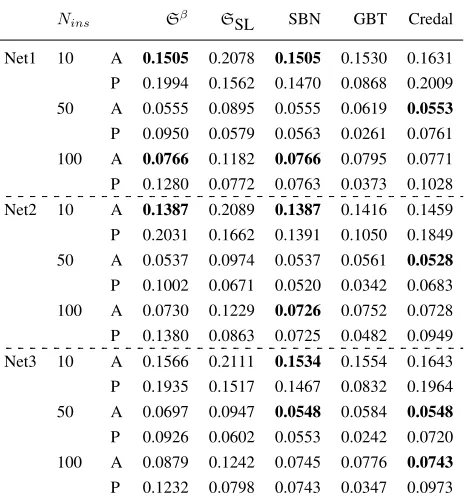
As before, Table 2 provides the root mean square error (RMSE) between the projected probabilities and the ground truth probabilities for all the inferred query variables for
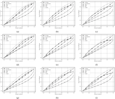
Nins = 10, 50, 100, together with the RMSE predicted by taking the square root of the average variances from the in-ferred marginal Beta distributions. Figure 3 plots the desired and actual significance levels for the confidence intervals (best closest to the diagonal).
(a) (b) (c)
Figure 2: Network structures tested where the exterior gray variables are directly observed and the remaining are queried: (a) Net1, a tree; (b) Net2, singly connected network with one node having two parents; (c) Net3, singly connected network with one node having three parents.
Nins Sβ SSL SBN GBT Credal
Net1 10 A 0.1505 0.2078 0.1505 0.1530 0.1631
P 0.1994 0.1562 0.1470 0.0868 0.2009
50 A 0.0555 0.0895 0.0555 0.0619 0.0553
P 0.0950 0.0579 0.0563 0.0261 0.0761
100 A 0.0766 0.1182 0.0766 0.0795 0.0771
P 0.1280 0.0772 0.0763 0.0373 0.1028
Net2 10 A 0.1387 0.2089 0.1387 0.1416 0.1459
P 0.2031 0.1662 0.1391 0.1050 0.1849
50 A 0.0537 0.0974 0.0537 0.0561 0.0528 P 0.1002 0.0671 0.0520 0.0342 0.0683
100 A 0.0730 0.1229 0.0726 0.0752 0.0728
P 0.1380 0.0863 0.0725 0.0482 0.0949
Net3 10 A 0.1566 0.2111 0.1534 0.1554 0.1643 P 0.1935 0.1517 0.1467 0.0832 0.1964
50 A 0.0697 0.0947 0.0548 0.0584 0.0548
P 0.0926 0.0602 0.0553 0.0242 0.0720
100 A 0.0879 0.1242 0.0745 0.0776 0.0743
P 0.1232 0.0798 0.0743 0.0347 0.0973
Table 2: RMSE for the queried variables in the various net-works: A stands for Actual, P for Predicted. Best results for the Actual RMSE in bold.
Sβcan also handle much more complex problems. Net3 re-sults are slightly worse due to approximations induced in the floating point operations used in the implementation: the more the connections of a node in the Bayesian network (e.g. node E in Figure 2c), the higher the number of operations in-volved in (7). A more accurate code engineering can address it. Consistently with Table 1, aProbLog withSβ has lower RMSE than with SSL and it underestimates its predicted
RMSE, while aProbLog withSSL overestimates it.
From visual inspection of Figure 3, it is evident that aProbLog with Sβ performs best in presence of high un-certainty (Nins “10). In presence of lower uncertainty,
in-stead, it underestimates its own prediction up to a desired confidence between 0.6 and 0.8, and overestimate it after. This is due to the fact that aProbLog computes the condi-tional distributions at the very end of the process and Sβ relies, in (21), on the assumption thatX andY are uncor-related. However, since the correlation betweenXandY is inversely proportional toaσ2
Xσ 2
Y, the lower the uncertainty, the less accurate our approximation.
5
Conclusion
We enabled the aProbLog approach to probabilistic logic programming to reason in presence of uncertain probabili-ties represented as Beta-distributed random variables. Other extensions to logic programming can handle uncertain prob-abilities by considering intervals of possible probprob-abilities (Ng and Subrahmanian 1992), similarly to the Credal net-work approach we compared against in Section 4; or by sampling random distributions, including ProbLog itself and cplint (Alberti et al. 2017) among others. Our approach does not require sampling or Monte Carlo computation, thus be-ing significantly more efficient.
Our experimental section shows that the proposed opera-tors outperform the standard subjective logic operaopera-tors and they are as good as the state-of-the-art approaches for un-certain probabilities in Bayesian networks while being able to handle much more complex problems. Moreover, in pres-ence of high uncertainty, which is our main research focus, the approximations we introduce in this paper are minimal, as Figures 3a, 3d, and 3g show, with the results of aProbLog withSβbeing very close to the diagonal.
(a) (b) (c)
(d) (e) (f)
(g) (h) (i)
Figure 3: Actual versus desired significance of bounds derived from the uncertainty for: (a) Net1 withNins “ 10; (b) Net1 withNins“50; (c) Net1 withNins“100; (d) Net2 withNins“10; (e) Net2 withNins“50; (f) Net2 withNins“100; (g) Net3 withNins “10; (h) Net3 withNins “50; (i) Net3 withNins“100. Best closest to the diagonal. In the figure,SL Beta represents aProbLog withSβ, andSL Operatorsrepresents aProbLog withS
SL.
A
Subjective Logic Operators of Sum,
Multiplication, and Division
Let us recall the following operators as defined in (Jøsang 2016). Let ωX “ xbX, dX, uX, aXy and ωY “ xbY, dY, uY, aYybe two subjective logic opinions, then: • the opinion about X YY (sum, ωX ‘SL ωY) is
de-fined asωXYY “ xbXYY, dXYY, uXYY, aXYYy, where
bXYY “ bX `bY, dXYY “
aXpdX´bYq`aYpdY´bXq
aX`aY , uXYY “aXuaXX``aaYYuY, andaXYY “aX`aY;
• the opinion about X ^ Y (product, ωX bSL ωY) is defined—under assumption of independence—as
ωX^Y “ xbX^Y, dX^Y, uX^Y, aX^Yy, wherebX^Y “
bXbY `p
1´aXqaYbXuY`aXp1´aYquXbY
1´aXaY ,dX^Y “dX`
dY´dXdY,uX^Y “uXuY`p
1´aYqbXuY`p1´aXquXbY
1´aXaY ,
andaX^Y “aXaY;
• the opinion about the division of X by Y,
X^rY (division, ωX mSL ωY) is defined as
ωX^rY “ xbX^rY, dX^rY, uX^rY, aX^rYy bX^rY =
aYpbX`aXuXq paY´aXqpbY`aYuYq´
aXp1´dXq
paY´aXqp1´dYq,dX^rY “
dX´dY
1´dY , uX^rY “
aYp1´dXq
paY´aXqp1´dYq ´
aYpbX`aXuXq
paY´aXqpbY`aYuYq, and aX^rY “
aX
aY,
subject to: aX ă aY; dX ě dY; bX ě aXp1´aYqp1´dXqbY
p1´aXqaYp1´dYq ;uXě
p1´aYqp1´dXquY
p1´aXqp1´dYq .
References
a web browser.Intelligenza Artificiale11(1):47–64. Allen, T. V.; Singh, A.; Greiner, R.; and Hooper, P. 2008. Quantifying the uncertainty of a belief net response: Bayesian error-bars for belief net inference. Artificial Intel-ligence172(4):483–513.
Anderson, R.; Hare, N.; and Maskell, S. 2016. Using a bayesian model for confidence to make decisions that con-sider epistemic regret. In19th International Conference on Information Fusion, 264–269.
Antonucci, A.; Karlsson, A.; and Sundgren, D. 2014. De-cision making with hierarchical credal sets. In Laurent, A.; Strauss, O.; Bouchon-Meunier, B.; and Yager, R. R., eds.,
Information Processing and Management of Uncertainty in Knowledge-Based Systems, 456–465.
De Raedt, L.; Kimmig, A.; and Toivonen, H. 2007. ProbLog: A probabilistic Prolog and its application in link discovery. In Proceedings of the 20th International Joint Conference on Artificial Intelligence, 2462–2467.
Dempster, A. P. 1968. A generalization of bayesian in-ference. Journal of the Royal Statistical Society. Series B (Methodological)30(2):205–247.
Eisner, J.; Goldlust, E.; and Smith, N. A. 2005. Compil-ing comp lCompil-ing: Practical weighted dynamic programmCompil-ing and the dyna language. InProceedings of the Conference on Human Language Technology and Empirical Methods in Natural Language Processing, HLT ’05, 281–290.
Fierens, D.; Van den Broeck, G.; Renkens, J.; Shterionov, D.; Gutmann, B.; Thon, I.; Janssens, G.; and De Raedt, L. 2015. Inference and learning in probabilistic logic programs using weighted Boolean formulas. Theory and Practice of Logic Programming15(03):358–401.
Gutmann, B.; Thon, I.; and De Raedt, L. 2011. Learning the parameters of probabilistic logic programs from interpreta-tions. InJoint European Conference on Machine Learning and Knowledge Discovery in Databases, 581–596.
Ivanovska, M.; Jøsang, A.; Kaplan, L.; and Sambo, F. 2015. Subjective networks: Perspectives and challenges. InProc. of the 4th International Workshop on Graph Structures for Knowledge Representation and Reasoning, 107–124. Jøsang, A.; Hayward, R.; and Pope, S. 2006. Trust network analysis with subjective logic. In Proceedings of the 29th Australasian Computer Science Conference-Volume 48, 85– 94.
Jøsang, A. 2016. Subjective Logic: A Formalism for Rea-soning Under Uncertainty. Springer.
Kaplan, L., and Ivanovska, M. 2016. Efficient subjective Bayesian network belief propagation for trees. In19th In-ternational Conference on Information Fusion, 1300–1307. Kaplan, L., and Ivanovska, M. 2018. Efficient belief propagation in second-order bayesian networks for singly-connected graphs. International Journal of Approximate Reasoning93:132–152.
Kimmig, A.; Van den Broeck, G.; and De Raedt, L. 2011. An algebraic prolog for reasoning about possible worlds. In
Proceedings of the Twenty-Fifth AAAI Conference on Artifi-cial Intelligence, 209–214.
Kleiter, G. D. 1996. Propagating imprecise probabilities in bayesian networks. Artificial Intelligence88(1):143 – 161. Minka, T. P. 2001. Expectation propagation for approximate bayesian inference. InProceedings of the Seventeenth Con-ference on Uncertainty in Artificial Intelligence, 362–369. Moglia, M.; Sharma, A. K.; and Maheepala, S. 2012. Multi-criteria decision assessments using subjective logic: Methodology and the case of urban water strategies. Jour-nal of Hydrology452-453:180–189.
Ng, R., and Subrahmanian, V. 1992. Probabilistic logic programming. Information and Computation101(2):150– 201.
Poole, D. 2000. Abducing through negation as failure: stable models within the independent choice logic. The Journal of Logic Programming44(1):5–35.
Sang, T.; Bearne, P.; and Kautz, H. 2005. Performing bayesian inference by weighted model counting. In Pro-ceedings of the 20th National Conference on Artificial Intel-ligence - Volume 1, 475–481.
Sato, T., and Kameya, Y. 2001. Parameter learning of logic programs for symbolic-statistical modeling. Journal of Ar-tificial Intelligence Research15(1):391–454.
Sato, T. 1995. A statistical learning method for logic programs with distribution semantics. In Proceedings of the 12th International Conference on Logic Programming (ICLP-95).
Sensoy, M.; Kaplan, L.; and Kandemir, M. 2018. Eviden-tial deep learning to quantify classification uncertainty. In
32nd Conference on Neural Information Processing Systems (NIPS 2018).
Smets, P. 1993. Belief functions: The disjunctive rule of combination and the generalized Bayesian theorem. Inter-national Journal of Approximate Reasoning9:1– 35. Von Neumann, J., and Morgenstern, O. 2007. Theory of games and economic behavior (commemorative edition). Princeton university press.
Zaffalon, M., and Fagiuoli, E. 1998. 2U: An exact interval propagation algorithm for polytrees with binary variables.