The Thirty-Third AAAI Conference on Artificial Intelligence (AAAI-19)
Graph Convolutional Networks for Text Classification
Liang Yao, Chengsheng Mao, Yuan Luo
∗ Northwestern UniversityChicago IL 60611
{liang.yao, chengsheng.mao, yuan.luo}@northwestern.edu
Abstract
Text classification is an important and classical problem in natural language processing. There have been a number of studies that applied convolutional neural networks (convolu-tion on regular grid, e.g., sequence) to classifica(convolu-tion. How-ever, only a limited number of studies have explored the more flexible graph convolutional neural networks (convolution on non-grid, e.g., arbitrary graph) for the task. In this work, we propose to use graph convolutional networks for text classi-fication. We build a single text graph for a corpus based on word co-occurrence and document word relations, then learn a Text Graph Convolutional Network (Text GCN) for the cor-pus. Our Text GCN is initialized with one-hot representation for word and document, it then jointly learns the embeddings for both words and documents, as supervised by the known class labels for documents. Our experimental results on mul-tiple benchmark datasets demonstrate that a vanilla Text GCN without any external word embeddings or knowledge outper-forms state-of-the-art methods for text classification. On the other hand, Text GCN also learns predictive word and docu-ment embeddings. In addition, experidocu-mental results show that the improvement of Text GCN over state-of-the-art compar-ison methods become more prominent as we lower the per-centage of training data, suggesting the robustness of Text GCN to less training data in text classification.
Introduction
Text classification is a fundamental problem in natural lan-guage processing (NLP). There are numerous applications of text classification such as document organization, news filtering, spam detection, opinion mining, and computa-tional phenotyping (Aggarwal and Zhai 2012; Zeng et al. 2018). An essential intermediate step for text classification is text representation. Traditional methods represent text with hand-crafted features, such as sparse lexical features (e.g., bag-of-words and n-grams). Recently, deep learning models have been widely used to learn text representa-tions, including convolutional neural networks (CNN) (Kim 2014) and recurrent neural networks (RNN) such as long short-term memory (LSTM) (Hochreiter and Schmidhuber 1997). As CNN and RNN prioritize locality and sequential-ity (Battaglia et al. 2018), these deep learning models can
∗
Corresponding Author
Copyright c2019, Association for the Advancement of Artificial Intelligence (www.aaai.org). All rights reserved.
capture semantic and syntactic information in local consec-utive word sequences well, but may ignore global word co-occurrence in a corpus which carries non-consecutive and long-distance semantics (Peng et al. 2018).
Recently, a new research direction called graph neural networks or graph embeddings has attracted wide atten-tion (Battaglia et al. 2018; Cai, Zheng, and Chang 2018). Graph neural networks have been effective at tasks thought to have rich relational structure and can preserve global structure information of a graph in graph embeddings.
In this work, we propose a new graph neural network-based method for text classification. We construct a single large graph from an entire corpus, which contains words and documents as nodes. We model the graph with a Graph Convolutional Network (GCN) (Kipf and Welling 2017), a simple and effective graph neural network that captures high order neighborhoods information. The edge between two word nodes is built by word co-occurrence information and the edge between a word node and document node is built using word frequency and word’s document frequency. We then turn text classification problem into a node classi-fication problem. The method can achieve strong classifica-tion performances with a small proporclassifica-tion of labeled docu-ments and learn interpretable word and document node em-beddings. Our source code is available at https://github.com/ yao8839836/text gcn. To summarize, our contributions are as follows:
• We propose a novel graph neural network method for text classification. To the best of our knowledge, this is the first study to model a whole corpus as a heterogeneous graph and learn word and document embeddings with graph neural networks jointly.
• Results on several benchmark datasets demonstrate that our method outperforms state-of-the-art text classification methods, without using pre-trained word embeddings or external knowledge. Our method also learns predictive word and document embeddings automatically.
Related Work
Traditional Text Classification
engineering, the most commonly used feature is the bag-of-words feature. In addition, some more complex features have been designed, such as n-grams (Wang and Manning 2012) and entities in ontologies (Chenthamarakshan et al. 2011). There are also existing studies on converting texts to graphs and perform feature engineering on graphs and sub-graphs (Luo, Uzuner, and Szolovits 2016; Rousseau, Kia-gias, and Vazirgiannis 2015; Skianis, Rousseau, and Vazir-giannis 2016; Luo et al. 2014; 2015). Unlike these methods, our method can learn text representations as node embed-dings automatically.
Deep Learning for Text Classification
Deep learning text classification studies can be catego-rized into two groups. One group of studies focused on models based on word embeddings (Mikolov et al. 2013; Pennington, Socher, and Manning 2014). Several recent studies showed that the success of deep learning on text clas-sification largely depends on the effectiveness of the word embeddings (Shen et al. 2018; Joulin et al. 2017; Wang et al. 2018). Some authors aggregated unsupervised word embeddings as document embeddings then fed these docu-ment embeddings into a classifier (Le and Mikolov 2014; Joulin et al. 2017). Others jointly learned word/document and document label embeddings (Tang, Qu, and Mei 2015; Wang et al. 2018). Our work is connected to these meth-ods, the major difference is that these methods build text representations after learning word embeddings while we learn word and document embeddings simultaneously for text classification.
Another group of studies employed deep neural networks. Two representative deep networks are CNN and RNN. (Kim 2014) used CNN for sentence classification. The archi-tecture is a direct application of CNNs as used in com-puter vision but with one dimensional convolutions. (Zhang, Zhao, and LeCun 2015) and (Conneau et al. 2017) designed character level CNNs and achieved promising results. (Tai, Socher, and Manning 2015), (Liu, Qiu, and Huang 2016) and (Luo 2017) used LSTM, a specific type of RNN, to learn text representation. To further increase the represen-tation flexibility of such models, attention mechanisms have been introduced as an integral part of models employed for text classification (Yang et al. 2016; Wang et al. 2016). Al-though these methods are effective and widely used, they mainly focus on local consecutive word sequences, but do not explicitly use global word co-occurrence information in a corpus.
Graph Neural Networks
The topic of Graph Neural Networks has received grow-ing attentions recently (Cai, Zheng, and Chang 2018; Battaglia et al. 2018). A number of authors generalized well-established neural network models like CNN that ap-ply to regular grid structure (2-d mesh or 1-d sequence) to work on arbitrarily structured graphs (Bruna et al. 2014; Henaff, Bruna, and LeCun 2015; Defferrard, Bresson, and Vandergheynst 2016; Kipf and Welling 2017). In their pi-oneering work, Kipf and Welling presented a simplified graph neural network model, called graph convolutional
networks (GCN), which achieved state-of-the-art classifi-cation results on a number of benchmark graph datasets (Kipf and Welling 2017). GCN was also explored in sev-eral NLP tasks such as semantic role labeling (Marcheggiani and Titov 2017), relation classification (Li, Jin, and Luo 2018) and machine translation (Bastings et al. 2017), where GCN is used to encode syntactic structure of sentences. Some recent studies explored graph neural networks for text classification (Henaff, Bruna, and LeCun 2015; Defferrard, Bresson, and Vandergheynst 2016; Kipf and Welling 2017; Peng et al. 2018; Zhang, Liu, and Song 2018). However, they either viewed a document or a sentence as a graph of word nodes (Defferrard, Bresson, and Vandergheynst 2016; Peng et al. 2018; Zhang, Liu, and Song 2018) or relied on the not-routinely-available document citation relation to con-struct the graph (Kipf and Welling 2017). In contrast, when constructing the corpus graph, we regard the documents and words as nodes (hence heterogeneous graph) and do not re-quire inter-document relations.
Method
Graph Convolutional Networks (GCN)
A GCN (Kipf and Welling 2017) is a multilayer neural net-work that operates directly on a graph and induces embed-ding vectors of nodes based on properties of their neigh-borhoods. Formally, consider a graph G = (V, E), where
V(|V| = n) andE are sets of nodes and edges, respec-tively. Every node is assumed to be connected to itself, i.e.,
(v, v)∈Efor anyv. LetX ∈Rn×mbe a matrix containing
allnnodes with their features, wheremis the dimension of the feature vectors, each rowxv ∈Rmis the feature vector
forv. We introduce an adjacency matrixAofGand its de-gree matrixD, whereDii =PjAij. The diagonal elements
ofAare set to1because of self-loops. GCN can capture in-formation only about immediate neighbors with one layer of convolution. When multiple GCN layers are stacked, in-formation about larger neighborhoods are integrated. For a one-layer GCN, the newk-dimensional node feature matrix
L(1) ∈
Rn×kis computed as
L(1)=ρ( ˜AXW0) (1)
whereA˜ = D−12AD− 1
2 is the normalized symmetric
ad-jacency matrix and W0 ∈ Rm×k is a weight matrix. ρis
an activation function, e.g. a ReLUρ(x) = max(0, x). As mentioned before, one can incorporate higher order neigh-borhoods information by stacking multiple GCN layers:
L(j+1)=ρ( ˜AL(j)Wj) (2)
wherejdenotes the layer number andL(0)=X.
Text Graph Convolutional Networks (Text GCN)
O35
O39
O42
O219
lung sarcoma Doppler
O3754
O276 O226
! "35
!("39)
!("42)
!("61)
Hidden Layers
Word Document Graph Word Document Representation
O61 O24
cardiac
,-.
/01
!023
45567
!("24)
!("226) !("219)
!("3754)
!("276)
R(cardiac)
R(T-cell) R(Doppler)
R(lung)
Document Class
T-cell
carcinoma
R(sarcoma)
R(carcinoma)
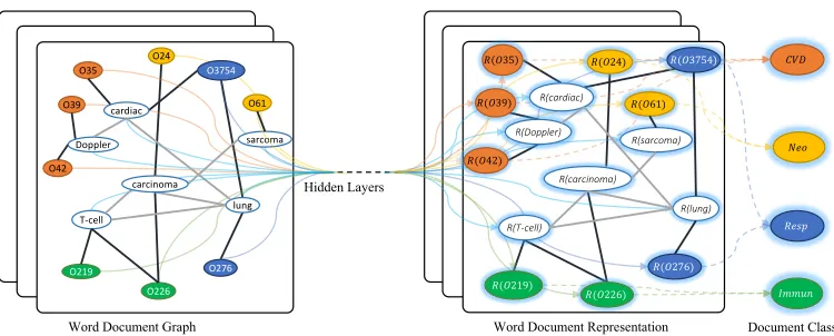
Figure 1: Schematic of Text GCN. Example taken from Ohsumed corpus. Nodes begin with “O” are document nodes, others are word nodes. Black bold edges are document-word edges and gray thin edges are word-word edges.R(x)means the repre-sentation (embedding) ofx. Different colors mean different document classes (only four example classes are shown to avoid clutter). CVD: Cardiovascular Diseases, Neo: Neoplasms, Resp: Respiratory Tract Diseases, Immun: Immunologic Diseases.
size) in a corpus. We simply set feature matrixX = I as an identity matrix which means every word or document is represented as a one-hot vector as the input to Text GCN. We build edges among nodes based on word occurrence in documents (document-word edges) and word co-occurrence in the whole corpus (word-word edges). The weight of the edge between a document node and a word node is the term frequency-inverse document frequency (TF-IDF) of the word in the document, where term frequency is the number of times the word appears in the document, inverse docu-ment frequency is the logarithmically scaled inverse frac-tion of the number of documents that contain the word. We found using TF-IDF weight is better than using term fre-quency only. To utilize global word co-occurrence informa-tion, we use a fixed size sliding window on all documents in the corpus to gather co-occurrence statistics. We employ point-wise mutual information (PMI), a popular measure for word associations, to calculate weights between two word nodes. We also found using PMI achieves better results than using word co-occurrence count in our preliminary exper-iments. Formally, the weight of edge between nodei and nodejis defined as
Aij =
PMI(i, j) i, jare words, PMI(i, j)>0
TF-IDFij iis document,jis word
1 i=j
0 otherwise
(3)
The PMI value of a word pairi, jis computed as
PMI(i, j) = log p(i, j)
p(i)p(j) (4)
p(i, j) =#W(i, j)
#W (5)
p(i) =#W(i)
#W (6)
where#W(i) is the number of sliding windows in a cor-pus that contain wordi,#W(i, j)is the number of sliding
windows that contain both word i andj, and #W is the total number of sliding windows in the corpus. A positive PMI value implies a high semantic correlation of words in a corpus, while a negative PMI value indicates little or no semantic correlation in the corpus. Therefore, we only add edges between word pairs with positive PMI values.
After building the text graph, we feed the graph into a sim-ple two layer GCN as in (Kipf and Welling 2017), the second layer node (word/document) embeddings have the same size as the labels set and are fed into asoftmaxclassifier:
Z=softmax( ˜AReLU( ˜AXW0)W1) (7)
whereA˜ = D−12AD− 1
2 is the same as in equation 1, and
softmax(xi) = Z1 exp(xi)withZ =Piexp(xi). The loss
function is defined as the cross-entropy error over all labeled documents:
L=− X
d∈YD
F X
f=1
YdflnZdf (8)
whereYD is the set of document indices that have labels
and F is the dimension of the output features, which is equal to the number of classes. Y is the label indicator matrix. The weight parametersW0 andW1can be trained
via gradient descent. In equation 7, E1 = AXW˜ 0
con-tains the first layer document and word embeddings and
E2 = ˜AReLU( ˜AXW0)W1contains the second layer
doc-ument and word embeddings. The overall Text GCN model is schematically illustrated in Figure 1.
Experiment
In this section we evaluate our Text Graph Convolutional Networks (Text GCN) on two experimental tasks. Specifi-cally we want to determine:
• Can our model achieve satisfactory results in text classifi-cation, even with limited labeled data?
• Can our model learn predictive word and document em-beddings?
Baselines. We compare our Text GCN with multiple state-of-the-art text classification and embedding methods as fol-lows:
• TF-IDF + LR: bag-of-words model with term frequency-inverse document frequency weighting. Logistic Regres-sion is used as the classifier.
• CNN: Convolutional Neural Network (Kim 2014). We ex-plored CNN-rand which uses randomly initialized word embeddings and CNN-non-static which uses pre-trained word embeddings.
• LSTM: The LSTM model defined in (Liu, Qiu, and Huang 2016) which uses the last hidden state as the rep-resentation of the whole text. We also experimented with the model with/without pre-trained word embeddings.
• Bi-LSTM: a bi-directional LSTM, commonly used in text classification. We input pre-trained word embeddings to Bi-LSTM.
• PV-DBOW: a paragraph vector model proposed by (Le and Mikolov 2014), the orders of words in text are ig-nored. We used Logistic Regression as the classifier.
• PV-DM: a paragraph vector model proposed by (Le and Mikolov 2014), which considers the word order. We used Logistic Regression as the classifier.
• PTE: predictive text embedding (Tang, Qu, and Mei 2015), which firstly learns word embedding based on het-erogeneous text network containing words, documents and labels as nodes, then averages word embeddings as document embeddings for text classification.
• fastText: a simple and efficient text classification method (Joulin et al. 2017), which treats the average of word/n-grams embeddings as document embeddings, then feeds document embeddings into a linear classifier. We evaluated it with and without bigrams.
• SWEM: simple word embedding models (Shen et al. 2018), which employs simple pooling strategies operated over word embeddings.
• LEAM: label-embedding attentive models (Wang et al. 2018), which embeds the words and labels in the same joint space for text classification. It utilizes label descrip-tions.
• Graph-CNN-C: a graph CNN model that operates con-volutions over word embedding similarity graphs (Deffer-rard, Bresson, and Vandergheynst 2016), in which Cheby-shev filter is used.
• Graph-CNN-S: the same as Graph-CNN-C but using Spline filter (Bruna et al. 2014).
• Graph-CNN-F: the same as Graph-CNN-C but using Fourier filter (Henaff, Bruna, and LeCun 2015).
Datasets. We ran our experiments on five widely used benchmark corpora including 20-Newsgroups (20NG), Ohsumed, R52 and R8 of Reuters 21578 and Movie Review (MR).
• The 20NG dataset1 (“bydate” version) contains 18,846
documents evenly categorized into 20 different cate-gories. In total, 11,314 documents are in the training set and 7,532 documents are in the test set.
• The Ohsumed corpus2 is from the MEDLINE database,
which is a bibliographic database of important medical lit-erature maintained by the National Library of Medicine. In this work, we used the 13,929 unique cardiovascular diseases abstracts in the first 20,000 abstracts of the year 1991. Each document in the set has one or more associ-ated categories from the 23 disease categories. As we fo-cus on single-label text classification, the documents be-longing to multiple categories are excluded so that 7,400 documents belonging to only one category remain. 3,357 documents are in the training set and 4,043 documents are in the test set.
• R52 and R83 (all-terms version) are two subsets of the Reuters 21578 dataset. R8 has 8 categories, and was split to 5,485 training and 2,189 test documents. R52 has 52 categories, and was split to 6,532 training and 2,568 test documents.
• MR is a movie review dataset for binary sentiment clas-sification, in which each review only contains one sen-tence (Pang and Lee 2005)4. The corpus has 5,331
posi-tive and 5,331 negaposi-tive reviews. We used the training/test split in (Tang, Qu, and Mei 2015)5.
We first preprocessed all the datasets by cleaning and tok-enizing text as (Kim 2014). We then removed stop words defined in NLTK6and low frequency words appearing less than 5 times for 20NG, R8, R52 and Ohsumed. The only exception was MR, we did not remove words after cleaning and tokenizing raw text, as the documents are very short. The statistics of the preprocessed datasets are summarized in Table 1.
Settings. For Text GCN, we set the embedding size of the first convolution layer as 200 and set the window size as 20. We also experimented with other settings and found that small changes did not change the results much. We tuned other parameters and set the learning rate as 0.02, dropout
1http://qwone.com/∼jason/20Newsgroups/
2
http://disi.unitn.it/moschitti/corpora.htm 3
https://www.cs.umb.edu/∼smimarog/textmining/datasets/
4http://www.cs.cornell.edu/people/pabo/movie-review-data/ 5
https://github.com/mnqu/PTE/tree/master/data/mr 6
Dataset # Docs # Training # Test # Words # Nodes # Classes Average Length
20NG 18,846 11,314 7,532 42,757 61,603 20 221.26
R8 7,674 5,485 2,189 7,688 15,362 8 65.72
R52 9,100 6,532 2,568 8,892 17,992 52 69.82
Ohsumed 7,400 3,357 4,043 14,157 21,557 23 135.82
MR 10,662 7,108 3,554 18,764 29,426 2 20.39
Table 1: Summary statistics of datasets.
Model 20NG R8 R52 Ohsumed MR
TF-IDF + LR 0.8319±0.0000 0.9374±0.0000 0.8695±0.0000 0.5466±0.0000 0.7459±0.0000 CNN-rand 0.7693±0.0061 0.9402±0.0057 0.8537±0.0047 0.4387±0.0100 0.7498±0.0070 CNN-non-static 0.8215±0.0052 0.9571±0.0052 0.8759±0.0048 0.5844±0.0106 0.7775±0.0072 LSTM 0.6571±0.0152 0.9368±0.0082 0.8554±0.0113 0.4113±0.0117 0.7506±0.0044 LSTM (pretrain) 0.7543±0.0172 0.9609±0.0019 0.9048±0.0086 0.5110±0.0150 0.7733±0.0089 Bi-LSTM 0.7318±0.0185 0.9631±0.0033 0.9054±0.0091 0.4927±0.0107 0.7768±0.0086 PV-DBOW 0.7436±0.0018 0.8587±0.0010 0.7829±0.0011 0.4665±0.0019 0.6109±0.0010 PV-DM 0.5114±0.0022 0.5207±0.0004 0.4492±0.0005 0.2950±0.0007 0.5947±0.0038 PTE 0.7674±0.0029 0.9669±0.0013 0.9071±0.0014 0.5358±0.0029 0.7023±0.0036 fastText 0.7938±0.0030 0.9613±0.0021 0.9281±0.0009 0.5770±0.0049 0.7514±0.0020 fastText (bigrams) 0.7967±0.0029 0.9474±0.0011 0.9099±0.0005 0.5569±0.0039 0.7624±0.0012 SWEM 0.8516±0.0029 0.9532±0.0026 0.9294±0.0024 0.6312±0.0055 0.7665±0.0063 LEAM 0.8191±0.0024 0.9331±0.0024 0.9184±0.0023 0.5858±0.0079 0.7695±0.0045 Graph-CNN-C 0.8142±0.0032 0.9699±0.0012 0.9275±0.0022 0.6386±0.0053 0.7722±0.0027 Graph-CNN-S – 0.9680±0.0020 0.9274±0.0024 0.6282±0.0037 0.7699±0.0014 Graph-CNN-F – 0.9689±0.0006 0.9320±0.0004 0.6304±0.0077 0.7674±0.0021 Text GCN 0.8634±0.0009 0.9707±0.0010 0.9356±0.0018 0.6836±0.0056 0.7674±0.0020
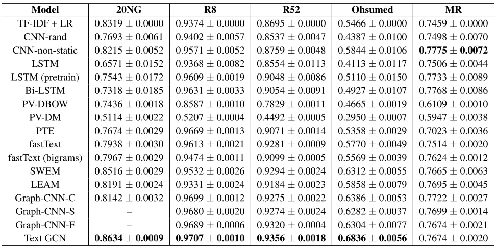
Table 2: Test Accuracy on document classification task. We run all models 10 times and report mean±standard deviation. Text GCN significantly outperforms baselines on 20NG, R8, R52 and Ohsumed based on studentt-test (p <0.05).
rate as 0.5,L2loss weight as 0. We randomly selected10%
of training set as validation set. Following (Kipf and Welling 2017), we trained Text GCN for a maximum of 200 epochs using Adam (Kingma and Ba 2015) and stop training if the validation loss does not decrease for 10 consecutive epochs. For baseline models, we used default parameter settings as in their original papers or implementations. For baseline models using pre-trained word embeddings, we used 300-dimensional GloVe word embeddings (Pennington, Socher, and Manning 2014)7.
Test Performance. Table 2 presents test accuracy of each model. Text GCN performs the best and significantly outper-forms all baseline models (p <0.05based on studentt-test) on four datasets, which showcases the effectiveness of the proposed method on long text datasets. For more in-depth performance analysis, we note that TF-IDF + LR performs well on long text datasets like 20NG and can outperform CNN with randomly initialized word embeddings. When pre-trained GloVe word embeddings are provided, CNN
7
http://nlp.stanford.edu/data/glove.6B.zip
This suggests that building word similarity graph using pre-trained word embeddings can preserve syntactic and seman-tic relations among words, which can provide additional in-formation in large external text data.
The main reasons why Text GCN works well are two fold: 1) the text graph can capture both document-word relations and global word-word relations; 2) the GCN model, as a spe-cial form of Laplacian smoothing, computes the new fea-tures of a node as the weighted average of itself and its second order neighbors (Li, Han, and Wu 2018). The la-bel information of document nodes can be passed to their neighboring word nodes (words within the documents), then relayed to other word nodes and document nodes that are neighbor to the first step neighboring word nodes. Word nodes can gather comprehensive document label informa-tion and act as bridges or key paths in the graph, so that label information can be propagated to the entire graph. However, we also observed that Text GCN did not outperform CNN and LSTM-based models on MR. This is because GCN ig-nores word orders that are very useful in sentiment classifi-cation, while CNN and LSTM model consecutive word se-quences explicitly. Another reason is that the edges in MR text graph are fewer than other text graphs, which limits the message passing among the nodes. There are only few document-word edges because the documents are very short. The number of word-word edges is also limited due to the small number of sliding windows. Nevertheless, CNN and LSTM rely on pre-trained word embeddings from external corpora while Text GCN only uses information in the target input corpus.
5 10 15 20 25 30 0.966 0.967 0.968 0.969 0.970 0.971 0.972
0.973 Text GCN
(a) R8
5 10 15 20 25 30 0.760
0.762 0.764 0.766 0.768
0.770 Text GCN
(b) MR
Figure 2: Test accuracy with different sliding window sizes.
0 50 100 150 200 250 300 0.935 0.940 0.945 0.950 0.955 0.960 0.965 0.970 0.975 Text GCN
(a) R8
0 50 100 150 200 250 300 0.7525 0.7550 0.7575 0.7600 0.7625 0.7650 0.7675
0.7700 Text GCN
(b) MR
Figure 3: Test accuracy by varying embedding dimensions.
Parameter Sensitivity. Figure 2 shows test accuracies with different sliding window sizes on R8 and MR. We can see that test accuracy first increases as window size becomes larger, but the average accuracy stops increasing when win-dow size is larger than 15. This suggests that too small
0.025 0.050 0.075 0.100 0.125 0.150 0.175 0.200 0.1 0.2 0.3 0.4 0.5 0.6 0.7 0.8 Text GCN CNN-non-static LSTM (pretrain) Graph-CNN-C TF-IDF + LR
(a) 20NG
0.025 0.050 0.075 0.100 0.125 0.150 0.175 0.200 0.2 0.3 0.4 0.5 0.6 0.7 0.8 0.9 1.0 Text GCN CNN-non-static LSTM (pretrain) Graph-CNN-C TF-IDF + LR
(b) R8
Figure 4: Test accuracy by varying training data proportions.
80 60 40 20 0 20 40 60 80 60 40 20 0 20 40 60 80
(a) Text GCN, 1st layer
75 50 25 0 25 50 75 75 50 25 0 25 50 75 100
(b) Text GCN, 2nd layer
60 40 20 0 20 40 60 80 60 40 20 0 20 40 60 (c) PV-DBOW
75 50 25 0 25 50 75 80 60 40 20 0 20 40 60 80 (d) PTE
Figure 5: The t-SNE visualization of test set document em-beddings in 20NG.
window sizes could not generate sufficient global word co-occurrence information, while too large window sizes may add edges between nodes that are not very closely related. Figure 3 depicts the classification performance on R8 and MR with different dimensions of the-first layer embeddings. We observed similar trends as in Figure 2. Too low dimen-sional embeddings may not propagate label information to the whole graph well, while high dimensional embeddings do not improve classification performances and may cost more training time.
Effects of the Size of Labeled Data. In order to evalu-ate the effect of the size of the labeled data, we tested sev-eral best performing models with different proportions of the training data. Figure 4 reports test accuracies with1%,5%,
word document graph preserves global word co-occurrence information.
Document Visualization. We give an illustrative visual-ization of the document embeddings leaned by Text GCN. We use t-SNE tool (Maaten and Hinton 2008) to visualize the learned document embeddings. Figure 5 shows the visu-alization of 200 dimensional 20NG test document embed-dings learned by GCN (first layer), PV-DBOW and PTE. We also show 20 dimensional second layer test document embeddings of Text GCN. We observe that Text GCN can learn more discriminative document embeddings, and the second layer embeddings are more distinguishable than the first layer.
comp.graphics sci.space sci.med rec.autos
jpeg space candida car
graphics orbit geb cars
image shuttle disease v12 gif launch patients callison
3d moon yeast engine
images prb msg toyota
rayshade spacecraft vitamin nissan polygon solar syndrome v8
pov mission infection mustang viewer alaska gordon eliot
Table 3: Words with highest values for several classes in 20NG. Second layer word embeddings are used. We show top 10 words for each class.
60 40 20 0 20 40 60 60
40 20 0 20 40 60
Figure 6: The t-SNE visualization of the second layer word embeddings (20 dimensional) learned from 20NG. We set the dimension with the largest value as a word’s label.
Word Visualization. We also qualitatively visualize word embeddings learned by Text GCN. Figure 6 shows the t-SNE visualization of the second layer word embeddings learned from 20NG. We set the dimension with the highest value as a word’s label. We can see that words with the same label are close to each other, which means most words are closely related to some certain document classes. We also show top 10 words with highest values under each class in Table 3. We note that the top 10 words are interpretable. For example, “jpeg”, “graphics” and “image” in column 1 can represent the meaning of their label “comp.graphics” well. Words in other columns can also indicate their label’s meaning.
Discussion. From experimental results, we can see the proposed Text GCN can achieve strong text classification re-sults and learn predictive document and word embeddings. However, a major limitation of this study is that the GCN model is inherently transductive, in which test document nodes (without labels) are included in GCN training. Thus Text GCN could not quickly generate embeddings and make prediction for unseen test documents. Possible solutions to the problem are introducing inductive (Hamilton, Ying, and Leskovec 2017) or fast GCN model (Chen, Ma, and Xiao 2018).
Conclusion and Future Work
In this study, we propose a novel text classification method termed Text Graph Convolutional Networks (Text GCN). We build a heterogeneous word document graph for a whole corpus and turn document classification into a node clas-sification problem. Text GCN can capture global word co-occurrence information and utilize limited labeled docu-ments well. A simple two-layer Text GCN demonstrates promising results by outperforming numerous state-of-the-art methods on multiple benchmark datasets.
In addition to generalizing Text GCN model to inductive settings, some interesting future directions include improv-ing the classification performance usimprov-ing attention mecha-nisms (Veliˇckovi´c et al. 2018) and developing unsupervised text GCN framework for representation learning on large-scale unlabeled text data.
Acknowledgments
This work is supported in part by NIH grant R21LM012618.
References
Aggarwal, C. C., and Zhai, C. 2012. A survey of text classi-fication algorithms. InMining text data. Springer. 163–222. Bastings, J.; Titov, I.; Aziz, W.; Marcheggiani, D.; and Simaan, K. 2017. Graph convolutional encoders for syntax-aware neural machine translation. InEMNLP, 1957–1967. Battaglia, P. W.; Hamrick, J. B.; Bapst, V.; Sanchez-Gonzalez, A.; Zambaldi, V.; Malinowski, M.; Tacchetti, A.; Raposo, D.; Santoro, A.; Faulkner, R.; et al. 2018. Rela-tional inductive biases, deep learning, and graph networks.
arXiv preprint arXiv:1806.01261.
Bruna, J.; Zaremba, W.; Szlam, A.; and LeCun, Y. 2014. Spectral networks and locally connected networks on graphs. InICLR.
Cai, H.; Zheng, V. W.; and Chang, K. 2018. A comprehen-sive survey of graph embedding: problems, techniques and applications. IEEE Transactions on Knowledge and Data Engineering30(9):1616–1637.
Chen, J.; Ma, T.; and Xiao, C. 2018. Fastgcn: Fast learning with graph convolutional networks via importance sampling. InICLR.
Conneau, A.; Schwenk, H.; Barrault, L.; and Lecun, Y. 2017. Very deep convolutional networks for text classification. In
EACL.
Defferrard, M.; Bresson, X.; and Vandergheynst, P. 2016. Convolutional neural networks on graphs with fast localized spectral filtering. InNIPS, 3844–3852.
Hamilton, W.; Ying, Z.; and Leskovec, J. 2017. Inductive representation learning on large graphs. In NIPS, 1024– 1034.
Henaff, M.; Bruna, J.; and LeCun, Y. 2015. Deep convo-lutional networks on graph-structured data. arXiv preprint arXiv:1506.05163.
Hochreiter, S., and Schmidhuber, J. 1997. Long short-term memory.Neural computation9(8):1735–1780.
Joulin, A.; Grave, E.; Bojanowski, P.; and Mikolov, T. 2017. Bag of tricks for efficient text classification. InEACL, 427– 431. Association for Computational Linguistics.
Kim, Y. 2014. Convolutional neural networks for sentence classification. InEMNLP, 1746–1751.
Kingma, D., and Ba, J. 2015. Adam: A method for stochastic optimization. InICLR.
Kipf, T. N., and Welling, M. 2017. Semi-supervised classi-fication with graph convolutional networks. InICLR. Le, Q., and Mikolov, T. 2014. Distributed representations of sentences and documents. InICML, 1188–1196.
Li, Q.; Han, Z.; and Wu, X. 2018. Deeper insights into graph convolutional networks for semi-supervised learning. InAAAI.
Li, Y.; Jin, R.; and Luo, Y. 2018. Classifying rela-tions in clinical narratives using segment graph convolu-tional and recurrent neural networks (seg-gcrns). Jour-nal of the American Medical Informatics AssociationDOI: 10.1093/jamia/ocy157.
Liu, P.; Qiu, X.; and Huang, X. 2016. Recurrent neural network for text classification with multi-task learning. In
IJCAI, 2873–2879. AAAI Press.
Luo, Y.; Sohani, A. R.; Hochberg, E. P.; and Szolovits, P. 2014. Automatic lymphoma classification with sentence subgraph mining from pathology reports. Journal of the American Medical Informatics Association21(5):824–832. Luo, Y.; Xin, Y.; Hochberg, E.; Joshi, R.; Uzuner, O.; and Szolovits, P. 2015. Subgraph augmented non-negative ten-sor factorization (santf) for modeling clinical narrative text.
Journal of the American Medical Informatics Association
22(5):1009–1019.
Luo, Y.; Uzuner, ¨O.; and Szolovits, P. 2016. Bridging se-mantics and syntax with graph algorithms —state-of-the-art of extracting biomedical relations.Briefings in bioinformat-ics18(1):160–178.
Luo, Y. 2017. Recurrent neural networks for classifying relations in clinical notes.Journal of biomedical informatics
72:85–95.
Maaten, L. v. d., and Hinton, G. 2008. Visualizing data using t-sne.JMLR9(Nov):2579–2605.
Marcheggiani, D., and Titov, I. 2017. Encoding sentences with graph convolutional networks for semantic role label-ing. InEMNLP, 1506–1515.
Mikolov, T.; Sutskever, I.; Chen, K.; Corrado, G. S.; and Dean, J. 2013. Distributed representations of words and phrases and their compositionality. InNIPS, 3111–3119. Pang, B., and Lee, L. 2005. Seeing stars: Exploiting class relationships for sentiment categorization with respect to rat-ing scales. InACL, 115–124.
Peng, H.; Li, J.; He, Y.; Liu, Y.; Bao, M.; Wang, L.; Song, Y.; and Yang, Q. 2018. Large-scale hierarchical text classifica-tion with recursively regularized deep graph-cnn. InWWW, 1063–1072.
Pennington, J.; Socher, R.; and Manning, C. 2014. Glove: Global vectors for word representation. InEMNLP, 1532– 1543.
Rousseau, F.; Kiagias, E.; and Vazirgiannis, M. 2015. Text categorization as a graph classification problem. In ACL, volume 1, 1702–1712.
Shen, D.; Wang, G.; Wang, W.; Renqiang Min, M.; Su, Q.; Zhang, Y.; Li, C.; Henao, R.; and Carin, L. 2018. Baseline needs more love: On simple word-embedding-based models and associated pooling mechanisms. InACL.
Skianis, K.; Rousseau, F.; and Vazirgiannis, M. 2016. Reg-ularizing text categorization with clusters of words. In
EMNLP, 1827–1837.
Tai, K. S.; Socher, R.; and Manning, C. D. 2015. Im-proved semantic representations from tree-structured long short-term memory networks. InACL, 1556–1566.
Tang, J.; Qu, M.; and Mei, Q. 2015. Pte: Predictive text em-bedding through large-scale heterogeneous text networks. In
KDD, 1165–1174. ACM.
Veliˇckovi´c, P.; Cucurull, G.; Casanova, A.; Romero, A.; Li`o, P.; and Bengio, Y. 2018. Graph attention networks. InICLR. Wang, S., and Manning, C. D. 2012. Baselines and bigrams: Simple, good sentiment and topic classification. InACL, 90– 94. Association for Computational Linguistics.
Wang, Y.; Huang, M.; Zhao, L.; et al. 2016. Attention-based lstm for aspect-level sentiment classification. InEMNLP, 606–615.
Wang, G.; Li, C.; Wang, W.; Zhang, Y.; Shen, D.; Zhang, X.; Henao, R.; and Carin, L. 2018. Joint embedding of words and labels for text classification. InACL, 2321–2331. Yang, Z.; Yang, D.; Dyer, C.; He, X.; Smola, A.; and Hovy, E. 2016. Hierarchical attention networks for document clas-sification. InNAACL, 1480–1489.
Zeng, Z.; Deng, Y.; Li, X.; Naumann, T.; and Luo, Y. 2018. Natural language processing for ehr-based computational phenotyping. IEEE/ACM transactions on computational bi-ology and bioinformatics10.1109/TCBB.2018.2849968. Zhang, Y.; Liu, Q.; and Song, L. 2018. Sentence-state lstm for text representation. InACL, 317–327.