The Thirty-Third AAAI Conference on Artificial Intelligence (AAAI-19)
Partial Label Learning with Self-Guided Retraining
Lei Feng,
1,2Bo An
11School of Computer Science and Engineering, Nanyang Technological University, Singapore
2Alibaba-NTU Singapore Joint Research Institute, Singapore
[email protected], [email protected]
Abstract
Partial label learning deals with the problem where each train-ing instance is assigned a set of candidate labels, only one of which is correct. This paper provides the first attempt to leverage the idea of self-training for dealing with par-tially labeled examples. Specifically, we propose a unified formulation with proper constraints to train the desired model and perform pseudo-labeling jointly. For pseudo-labeling, un-like traditional self-training that manually differentiates the ground-truth label with enough high confidence, we intro-duce the maximum infinity norm regularization on the model-ing outputs to automatically achieve this consideratum, which results in a convex-concave optimization problem. We show that optimizing this convex-concave problem is equivalent to solving a set of quadratic programming (QP) problems. By proposing an upper-bound surrogate objective function, we turn to solving only one QP problem for improving the op-timization efficiency. Extensive experiments on synthesized and real-world datasets demonstrate that the proposed ap-proach significantly outperforms the state-of-the-art partial label learning approaches.
Introduction
In partial label (PL) learning, each training example is rep-resented by a single instance (feature vector) while asso-ciated with a set of candidate labels, only one of which is the ground-truth label. This learning paradigm is also termed assuperset label learning(Liu and Dietterich 2012; 2014; H¨ullermeier and Cheng 2015; Gong et al. 2018) or
ambiguous label learning (H¨ullermeier and Beringer 2006; Zeng et al. 2013; Chen et al. 2014; Chen, Patel, and Chel-lappa 2017). Since manually labeling the ground-truth label of each instance could incur unaffordable monetary or time cost, partial label learning has various application domains, such as web mining (Luo and Orabona 2010), image anno-tation (Cour, Sapp, and Taskar 2011; Zeng et al. 2013), and ecoinformatics (Liu and Dietterich 2012).
Formally, letX ∈Rnbe then-dimensional feature space
and Y = {1,2,· · ·, l} be the corresponding label space with l labels. Suppose the PL training set is denoted by D = {xi, Si}im=1 wherexi ∈ X is ann-dimensional fea-ture vector andSi denotes the candidate label set. The key
Copyright c2019, Association for the Advancement of Artificial Intelligence (www.aaai.org). All rights reserved.
assumption of partial label learning lies in that the ground-truth label for xi is concealed in its candidate label set
Si. The task of partial label learning is to learn a function
f :X → Y from the PL training setD, to correctly predict the label of a test instance.
Obviously, the available labeling information in the PL training set is ambiguous, as the ground-truth label is con-cealed in the candidate label set. Hence the key for accom-plishing the task of learning from PL examples is how to disambiguate the candidate labels. Based on the employed strategy, existing approaches can be roughly grouped into two categories, including the average-based strategy and the identification-based strategy. The average-based strategy as-sumes that each candidate label makes equal contributions to the model training, and the prediction is made by averag-ing their modelaverag-ing outputs (H¨ullermeier and Beraverag-inger 2006; Cour, Sapp, and Taskar 2011; Zhang, Zhou, and Liu 2016). The identification-based strategy considers the ground-truth label as a latent variable, which is identified by an itera-tive refining procedure (Jin and Ghahramani 2003; Nguyen and Caruana 2008; Liu and Dietterich 2012; Yu and Zhang 2016). Although these approaches are able to extract the rel-ative labeling confidence of each candidate label, they fail to reflect the mutually exclusive relationships among different candidate labels.
Motivated by self-training that takes into account such mutually exclusive relationships by directly labeling an un-labeled instance with enough high confidence, this paper gives the first attempt to leverage the similar idea to deal with PL instances. A straightforward method is to first apply a multi-output model on the PL examples, then pick up the candidate label with enough high confidence as the ground-truth label, finally retrain the model on the resulting data. This process is repeated until no PL examples exist, or no PL examples can be picked up as the ground-truth label. Al-though this method is intuitive, the model learned from PL examples are probably hard to directly identify the ground-truth label in accordance with the modeling outputs, as can-didate label sets exist. Furthermore, the incorrectly identified labels could have contagiously negative impacts on the final predictions.
proper constraints to train the desired model and perform pseudo-labeling jointly. Unlike traditional self-training that manually differentiates the ground-truth label with enough high confidence, we introduce the maximum infinity norm regularization on the modeling outputs to automatically per-form pseudo-labeling. In this way, the pseudo labels are de-cided by balancing the minimum approximation loss and the maximum infinity norm. To optimize the objective function, a convex-concave problem is encountered, as a result of the maximum infinity norm regularization. We show that solv-ing this convex-concave problem is equivalent to solvsolv-ing a set of quadratic programming problems. By proposing an upper-bound surrogate objective function, we turn to solving only one quadratic programming problem for improving the optimization efficiency. Extensive experiments on a number of synthesized and real-world datasets clearly demonstrate the advantage of the proposed approach.
Related Work
Due to the difficulty in dealing with ambiguous labeling information of PL examples, there are only two general strategies to disambiguate the candidate labels, including the average-based strategy and the identification-based strategy. The average-based strategy treats each candidate label equally in the model training phase. Following this strategy, some instance-based approaches predict the labely of the test instancexby averaging the candidate labels of its neigh-bors (H¨ullermeier and Beringer 2006; Zhang and Yu 2015), i.e.,arg maxy∈YP
xi∈N(x)I(yi∈Si)whereN(x)denotes the neighbors of instancex. Besides, some parametric ap-proaches adopt a parametric modelF(xi, y;θ)(Cour, Sapp, and Taskar 2011; Zhang, Zhou, and Liu 2016) that differen-tiates the average modeling output of the candidate labels, i.e., |S1i|P
y∈SiF(xi, y;θ)from that of the non-candidate
labels, i.e.,F(xi,yˆ;θ) (ˆy∈Sˆi), whereSˆidenotes the non-candidate label set. Although this strategy is intuitive, an ob-vious drawback is that the modeling output of the ground-truth label may be overwhelmed by the distractive outputs of the false positive labels.
The identification-based strategy considers the ground-truth label as a latent variable, and assumes certain parametric model F(x, y;θ) where the ground-truth label is identified by arg maxy∈SiF(xi, y;θ). Gen-erally, the specific objective function is optimized on the basis of the maximum likelihood criterion: max(Pmi=1log(P
y∈Si 1
|Si|F(xi, y;θ))) (Jin and Ghahra-mani 2003; Liu and Dietterich 2012) or the maximum margin criterion: max(Pmi=1(maxy∈SiF(xi, y;θ) −
maxyˆ∈SˆiF(xi,yˆ;θ))) (Nguyen and Caruana 2008; Yu and Zhang 2016). One potential drawback of this strat-egy lies in that instead of recovering the ground-truth label, the differentiated label may turn out to be false positive, which could severely disrupt the subsequent model training. Self-training is a commonly used technique for semi-supervised learning (Zhu and Goldberg 2009), which is characterized by the fact that the learning process uses its own predictions to teach itself. It has the advantage of taking into account the mutually exclusive relationships among
la-bels by directly labeling an unlabeled instance with enough high confidence. Despite of its simplicity, the early mistakes could be exaggerated by further generating incorrectly la-beled data. It is going to be even worse in the PL setting, as the ground-truth label is concealed in the candidate label set. By alleviating the negative effects of self-training with a unified formulation, a novel partial label learning ap-proach following the identification-based strategy will be in-troduced in the next section.
The Proposed Approach
Following the notations in Introduction, we denote byX= [x1,· · ·,xm]> ∈ Rm×n the instance matrix and Y =
[y1,· · ·,ym]> ∈ {0,1}m×lthe corresponding label matrix, whereyij = 1means that thej-th label is a candidate label of the i-th instance xi, otherwise the j-th label is a non-candidate label. By adopting the identification-based strat-egy, we also regard the ground-truth label as latent variable, and denote byP = [p1,· · · ,pm]> ∈ [0,1]m×lthe confi-dence matrix wherepij represents the confidence (probabil-ity) of thej-th label being the ground-truth label of thei-th instance.
Unlike self-training that takes into account the mutu-ally exclusive relationships among the candidate labels by performing deterministic pseudo-labeling, we introduce the maximum infinity norm regularization to automati-cally achieve this consideratum. A unified formulation with proper constraints is proposed as follows:
min m X
i=1
(L(xi,pi, f)−λkpik∞) +βΩ(f)
s.t. 0≤pij ≤yij, ∀i∈[m], ∀j∈[l] (1)
Xl
j=1pij = 1, ∀i∈[m]
in-finity norm regularization, the confidences of other candi-date labels will be naturally reduced.
To instantiate the above formulation, we adopt the widely used squared loss, i.e.,L(xi,pi, f) = kf(xi)−pik
2 2.
Be-sides, we employ the simple linear modelf(xi) =W>xi+
bwhere W,bare model parameters. A kernel extension for the general nonlinear case will be introduced in the later section. To control the model parameter, we simply adopt the common squared Frobenius norm ofW, i.e.,kWk2F. To sum up, the final optimization problem is presented as fol-lows:
min
P,W,b
m X
i=1
(W>xi+b−pi
2
2−λkpik∞) +βkWk 2
F
s.t. 0≤pij ≤yij, ∀i∈[m], ∀j∈[l] (2)
Xl
j=1pij = 1, ∀i∈[m]
Optimization
Problem (2) can be solved by alternating minimization, which enable us to optimize one variable with other vari-ables fixed. This process is repeated until convergence or the maximum number of iterations is reached.
Updating
W
and
b
WithPfixed, problem (2) with respective toWandbcan be compactly stated as follows:
min
W,b
XW+1b>−P
2
F +βkWk
2
F (3)
where1 denotes the vector with all components set to 1. Setting the gradient with respect toWandbto 0, the closed-form solutions can be easily obtained:
W= (X>X+βI−X
>11>X
m )
−1(X>P−X>11>P
m )
b= 1 m(P
>1−W>X>1) (4)
Kernel Extension To deal with the nonlinear case, the above linear learning model can be easily extended to a kernel-based nonlinear model. To achieve this, we utilize a feature mapping φ(·) : Rn → RH to map the
orig-inal feature space x ∈ Rn to some higher (maybe infi-nite) dimensional Hilbert spaceφ(x) ∈ RH. By
represen-tor theorem (Sch¨olkopf, Smola, and others 2002),W can be represented by a linear combination of input variables, i.e.,W = φ(X)>A whereA ∈ Rm×l stores the
combi-nation weights of instances. Henceφ(X)W =KAwhere
K ∈φ(X)φ(X)> ∈Rm×mis the kernel matrix with each
element defined bykij = φ(xi)>φ(xj) = κ(xi,xj), and
κ(·,·) denotes the kernel function. In this paper, Gaussian kernel function κ(xi,xj) = exp(− kxi−xjk
2 2/(2σ
2))is
employed withσ set to the averaged pairwise distances of instances. By incorporating such kernel extension, problem (3) can be presented as follows:
min
A,b
KA+1b>−P
2
F+βtr(A
>KA) (5)
wheretr(·)is the trace operator. Setting the gradient with re-spect toAandbto 0, the closed-form solutions are reported as:
A= (K+βI−11
>K
m )
−1(P−11>P
m )
b= 1 m(P
>1−A>K>1) (6)
By adopting this kernel extension, we choose to update the parametersAandbthroughout this paper.
Updating
P
With A and b fixed, the modeling output matrix Q = [q1,· · ·,qm]> ∈ Rm×l is denoted by Q = φ(X)W+ 1b> =KA+1b>, problem (2) reduces to:
min
P
m X
i=1
(kpi−qik
2
2−λkpik∞)
s.t. 0≤pij ≤yij, ∀i∈[m], ∀j∈[l] (7)
Xl
j=1pij = 1, ∀i∈[m]
Obviously, we can solve problem (7) by solvingm indepen-dent problems, one for each example. We further denote by
OPthe minimum loss of the problem for thei-th example:
OP= min
pi
kpi−qik
2
2−λkpik∞
s.t. 1>pi= 1 (8)
0≤pi≤yi
Here, problem (8) is a constrained convex-concave problem, as the first term is convex while the second term is concave. Instead of using traditional time-consuming convex-concave procedure (Yuille and Rangarajan 2003) to solve this prob-lem, we show that optimizing this problem is equivalent to solvinglindependent QP problems, each for one label. We denoted byOPI(j)the minimum loss of the problem for the
j-th label:
OPI(j) = min
pi
kpi−qik
2 2−λpij
s.t. pik≤pij, ∀k∈[l] (9)
1>pi= 1
0≤pi≤yi
Theorem 1. OP= minj∈[l]OPI(j).
Proof. It is obvious that there must existj ∈ [l]such that
pij = kpik∞ and the optimum loss OP of problem (8) can be obtained. In addition, if pij = kpik∞
coinciden-tally holds, then OPI(j) = OP, as in such case, problem (9) is equivalent to problem (8). While ifpij6=kpik∞, then OPI(j)>OP. HenceOP= minj∈[l]OPI(j).
Thus, we propose a surrogate objective function to upper bound the loss incurred by problem (8). Specifically, we se-lect the candidate labeljwith the maximal modeling output byj = arg maxj∈Siqij whereSiis the candidate label set containing the indices of candidate labels of the instancexi. The proposed surrogate objective function is given as:
OPS= min
pi
kpi−qik
2 2−λpij
s.t. qik≤qij, ∀k∈Si, ∃j∈Si (10)
pik≤pij, ∀k∈[l]
1>pi= 1
0≤pi≤yi
Note that the difference between problem (10) and prob-lem (9) lies in that probprob-lem (10) adds a constraint to se-lect the label j with the maximal modeling output. Un-like problem (9) that considers the possibility of each la-bel being the ground-truth lala-bel, problem (10) directly as-sumes the candidate labeljwith the maximal modeling out-putj = arg maxj∈Siqij to be the label that is most likely the ground-truth label. This assumption coincides with self-training, which also considers the label with the maximal modeling output as the ground-truth label. Different from self-training that manually performs deterministic pseudo-labeling, our approach aims to automatically enlarge the confidence of the label with the maximal modeling output as much as possible by balancing the two terms in problem (10). In this way, we not only avoid the opinionated mistakes by self-training, but also take into account the mutually ex-clusive relationships among candidate labels.
Theorem 2. OP≤OPS.
Proof. From the formulation of problem (10) and prob-lem (9), it is easy to see that OPS ∈ {OPI(j)|j ∈
Si}. Since Si ⊂ [l], OPS ∈ {OPI(j)|j ∈ [l]}. Which means,minj∈[l]OPI(j)≤OPS. Using Theorem (1),OP=
minj∈[l]OPI(j)≤OPS.
Theorem (2) shows thatOPSof problem (10) is an upper bound of the lossOPincurred by problem (8). Hence we can choose to optimize problem (10) for efficiency, as only one QP problem is involved. Such problem can be easily solved by any off-the-shelf QP tools.
After the completion of the optimization process, the pre-dicted labelyeof the text instancexeis given as:
e
y= arg max j∈[l]
m X
i=1
aijκ(ex,xi) +bj (11)
The pseudo code of SURE is presented in Algorithm 1.
Experiments
Comparing Algorithms
To demonstrate the effectiveness of SURE, we conduct ex-tensive experiments to compare SURE with six state-of-the-art pstate-of-the-artial label learning algorithms, each configured with suggested parameters according to the respective literature:
Algorithm 1The SURE Algorithm
Inputs:
D: the PL training setD={(X,Y)}
λ, β: the regularization parameters
e
x: the unseen test instance Output:
e
y: the predicted label for the test instanceex
1: construct the kernel matrixK= [κ(xi,xj)]m×m; 2: initializeP=Y;
3: repeat
4: updateA= [aij]m×landb= [bj]laccording to (6);
5: updateQ=KA+1b>;
6: calculatePby solving (10) with a general QP proce-dure for each training example;
7: until convergence or the maximum number of itera-tions.
8: return the predicted labelyeaccording to (11).
• PLKNN (H¨ullermeier and Beringer 2006): a k-nearest neighbor approach that makes predictions by averaging the labeling information of neighboring examples [sug-gested configuration:k∈ {5,6,· · ·,10}];
• CLPL (Cour, Sapp, and Taskar 2011): a convex formu-lation that deals with PL examples by transforming par-tial label learning problem to binary learning problem via feature mapping [suggested configuration: SVM with squared hinge loss];
• IPAL (Zhang and Yu 2015): an instance-based approach that disambiguates candidate labels by an adapted la-bel propagation scheme. [suggested configuration: α ∈ {0,0.1,· · ·,1},k∈ {5,6,· · · ,10}];
• PLSVM (Nguyen and Caruana 2008): a maximum mar-gin approach that learns from PL examples by optimiz-ing margin-based objective function [suggested configu-ration:λ∈ {10−3,10−2,· · ·,103}];
• PALOC (Wu and Zhang 2018): an approach that adapts one-vs-one decomposition strategy to enable binary de-composition for learning from PL examples [suggested configuration:µ= 10];
• LSBCMM (Liu and Dietterich 2012): a maximum likeli-hood approach that learns from PL examples via mixture models [suggested configuration:L=d10 log2(l)e].
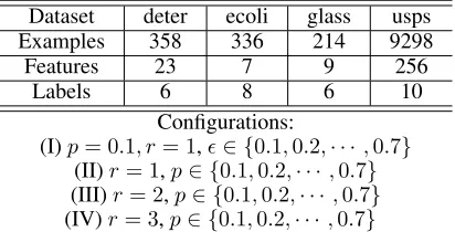
Table 1: Characteristics of the controlled UCI datasets.
Dataset deter ecoli glass usps
Examples 358 336 214 9298
Features 23 7 9 256
Labels 6 8 6 10
Configurations:
(I)p= 0.1, r= 1,∈ {0.1,0.2,· · ·,0.7} (II)r= 1,p∈ {0.1,0.2,· · · ,0.7} (III)r= 2,p∈ {0.1,0.2,· · ·,0.7} (IV)r= 3,p∈ {0.1,0.2,· · · ,0.7}
Controlled UCI Datasets
The characteristics of 4 controlled UCI datasets are reported in Table 1. Following the widely-used controlling proto-col (Cour, Sapp, and Taskar 2011; Liu and Dietterich 2012; Zhang and Yu 2015; Wu and Zhang 2018; Feng and An 2018; Wang and Zhang 2018), each UCI dataset can be used to generate artificial partial label datasets. There are three controlling parameters p, r and where p controls the proportion of PL examples, r controls the number of false positive labels, andcontrols the probability of a spe-cific false positive label occurring with the ground-truth la-bel. As shown in Table 1, there are 4 configurations, each corresponding to 7 results. Hence we can totally generate 4×4×7 = 112different artificial partial label datasets.
Figure 1 shows the classification accuracy of each algo-rithm asranges from 0.1 to 0.7 whenp= 0.1andr = 1 (Configuration (I)). In this setting, a specific label is selected as the coupled label that co-occurs with the ground-truth la-bel with probability , and any other label would be ran-domly chosen to be a false positive label with probability 1−. Figures 2, 3, and 4 illustrate the classification accuracy of each algorithm aspranges from 0.1 to 0.7 whenr= 1,2, and 3 (Configuration (II), (III), and (IV)), respectively. In these three settings,rextra labels are randomly chosen to be the false positive labels. That is, the number of candidate labels for each instance isr+ 1. As shown in Figures 1, 2, 3, and 4, SURE outperforms other comparing algorithms in general. To further statistically compare SURE with other algorithms, the detailed win/tie/loss counts between SURE and the comparing algorithms are recorded in Table 2. Out of the 112 results, it is easy to observe that:
• SURE achieves superior or at least comparable perfor-mance against PLKNN and PLSVM in all cases.
• SURE achieves superior performance against CLPL and LSCMM in 72.3% and 58.9% cases while outperformed by them in only 4.5% and 1.8% cases, respectively.
• SURE outperforms IPAL and PALOC in 50.9% and 63.4% cases while outperformed by them in only 5.4% and 2.7% cases, respectively.
In summary, the effectiveness of SURE on controlled UCI datasets is demonstrated.
Table 2: Win/tie/loss (t-test at 0.05 significance level for two independent samples) counts on the controlled UCI datasets between SURE and the comparing algorithms.
PLKNN CLPL IPAL PLSVM PALOC LSBCMM (I) 24/4/0 21/6/1 14/11/3 21/7/0 20/8/0 14/14/0 (II) 24/4/0 19/7/2 15/13/0 24/4/0 17/10/1 17/10/1 (III) 24/4/0 21/6/1 14/13/1 25/3/0 17/10/1 19/9/0 (IV) 25/3/0 20/7/1 14/12/2 27/1/0 17/10/1 16/11/1 Total 97/15/0 81/26/5 57/49/6 97/15/0 71/38/3 66/44/2
Real-World Datasets
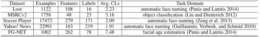
Table 3 reports the characteristics of real-world partial la-bel datasets1including Lost (Cour, Sapp, and Taskar 2011), MSRCv2 (Liu and Dietterich 2012), Soccer Player (Zeng et al. 2013), Yahoo! News (Guillaumin, Verbeek, and Schmid 2010), and FG-NET (Panis and Lanitis 2014). These real-world partial label datasets are from several task domains. For automatic face naming (Lost, Soccer Player, and Ya-hoo! News), each face (instance) is cropped from an im-age or a video frame, and the names appearing on the cor-responding captions or subtitles are taken as candidate la-bels. Forfacial age estimation(FG-NET), human faces are regarded as instances while ages annotated by crowdsourc-ing labelers serve as candidate labels. Forobject classifica-tion(MSRCv2), each image segment is considered as an in-stance, and objects appearing in the same image are taken as candidate labels. The average number of candidate labels (Avg. CLs) per instance is also reported in Table 3.
Table 4 reports the mean classification accuracy as well as the standard deviation of each algorithm on each real-world dataset. Note that the average number of candidate labels (Avg. CLs) of FG-NET dataset is quite large, which results in an extremely low classification accuracy of each algorithm. For better evaluation of this facial age estima-tion task, we employ convenestima-tional mean absolute error (MAE) (Zhang, Zhou, and Liu 2016) to conduct two extra experiments. Specifically, for FG-NET (MAE3/MAE5), a test example is considered correctly classified if the MAE between the predicted age and the ground-truth age is no more than 3/5 years. As shown in Table 4, we can observe that:
• SURE significantly outperforms PLKNN on all the real-world datasets.
• Out of the 42 cases (6 comparing algorithms and 7 datasets), SURE significantly outperforms all the compar-ing algorithms in 78.6% cases, and achieves competitive performance in 21.4% cases.
• It is worth noting that SURE is never significantly outper-formed by any comparing algorithms.
These experimental results on real-world datasets also demonstrate the effectiveness of SURE.
Further Analysis
1
(a) ecoli (b) deter (c) glass (d) usps
Figure 1: Classification performance on controlled UCI datasets withranging from 0.1 to 0.7 (p= 1, r= 1).
(a) ecoli (b) deter (c) glass (d) usps
Figure 2: Classification performance on controlled UCI datasets withpranging from 0.1 to 0.7 (r= 1).
(a) ecoli (b) deter (c) glass (d) usps
Figure 3: Classification performance on controlled UCI datasets withpranging from 0.1 to 0.7 (r= 2).
(a) ecoli (b) deter (c) glass (d) usps
Figure 4: Classification performance on controlled UCI datasets withpranging from 0.1 to 0.7 (r= 3).
Table 3: Characteristics of real-world partial label datasets.
Dataset Examples Features Labels Avg. CLs Task Domain
Lost 1122 108 16 2.23 automatic face naming(Panis and Lanitis 2014)
MSRCv2 1758 48 23 3.16 object classification(Liu and Dietterich 2012) Soccer Player 17472 279 171 2.09 automatic face naming(Zeng et al. 2013)
Yahoo! News 22991 163 219 1.91 automatic face naming(Guillaumin, Verbeek, and Schmid 2010) FG-NET 1002 262 78 7.48 facial age estimation(Panis and Lanitis 2014)
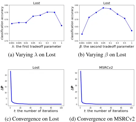
Parameter Sensitivity Analysis There are two tradeoff parametersλandβ for SURE, which should be manually
searched in advance. Hence this section studies howλandβ
Table 4: Classification accuracy of each algorithm on the real-world datasets. Furthermore,•/◦indicates whether SURE is statistically superior/inferior to the comparing algorithm (t-test at 0.05 significance level for two independent samples).
SURE PLKNN CLPL IPAL PLSVM PALOC LSBCMM
Lost 0.781±0.039 0.432±0.051• 0.742±0.038• 0.678±0.053• 0.729±0.042• 0.629±0.056• 0.693±0.035• MSRCv2 0.515±0.027 0.417±0.034• 0.413±0.041• 0.529±0.039 0.461±0.046• 0.479±0.042• 0.473±0.037• Soccer Player 0.533±0.017 0.495±0.018• 0.368±0.010• 0.541±0.016 0.464±0.011• 0.537±0.015 0.498±0.017• Yahoo! News 0.644±0.015 0.483±0.011• 0.462±0.009• 0.609±0.011• 0.629±0.010• 0.625±0.005• 0.645±0.005
FG-NET 0.078±0.021 0.039±0.018• 0.063±0.027 0.054±0.030• 0.063±0.029 0.065±0.019 0.059±0.025• FG-NET(MAE3) 0.458±0.024 0.269±0.045• 0.458±0.022 0.362±0.034• 0.356±0.022• 0.435±0.018• 0.382±0.029• FG-NET(MAE5) 0.615±0.019 0.438±0.053• 0.596±0.017• 0.540±0.033• 0.479±0.016• 0.609±0.043 0.532±0.038•
(a) Varyingλon Lost (b) Varyingβon Lost
(c) Convergence on Lost (d) Convergence on MSRCv2
Figure 5: Parameter sensitivity and convergence analysis for SURE. (a) Sensitivity analysis of λon Lost; (b) Sensitiv-ity analysis ofβ on MSRCv2; (c) Convergence analysis on Lost; (d) Convergence analysis on MSRCv2.
vary one parameter, while keeping the other fixed at the best setting. Figures 5(a) and 5(b) show the performance of SURE on the Lost dataset given different values ofλandβ
respectively. Note thatλcontrols the importance of the max-imum infinity norm regularization. When λis very small, the mutually exclusive relationships among labels are hardly considered, thus the classification accuracy would be at a low level. Asλincreases, we start to take into consideration such exclusive relationships, and the classification accuracy increases. However, ifλis sufficiently large, the classifica-tion accuracy will drop dramatically. This is because when we overly concentrate on the mutually exclusive relation-ships among labels, we will directly regard the candidate la-bel that has the maximal modeling output as the ground-truth label. Since to maximize the infinity normkpk∞is overly important, the approximation loss will be totally ignored. From the above, we can draw a conclusion that it would be better to balance the approximation loss and the mutually ex-clusive relationships among labels. Such conclusion clearly comfirms the effectiveness of the SURE approach. Another
tradeoff parameterβ aims to control the model complexity. The classification accuracy curve of varyingβobviously ac-cords with our cognition that it is important to balance be-tween overfitting and underfitting.
Illustration of Convergence We illustrate the convergece of SURE by using the difference of the optimization variable P between two successive iterations (∆P =
P(t+1)−P(t)
F). Figure 5(c) and 5(d) show the conver-gence curves of SURE on Lost and MSRCv2 respectively. It is apparent that∆Pgradually decreases to 0 as the number of iterationstincreases. Hence the convergence of SURE is demonstrated.
Conclusion
In this paper, we utilize the idea of self-training to exag-gerate the mutually exclusive relationships among candidate labels for further enhancing partial label learning perfor-mance. Instead of manually performing pseudo-labeling af-ter model training, we propose a unified formulation (named SURE) with the maximum infinity norm regularization to train the desired model and perform pseudo-labeling jointly. Extensive experimental results demonstrate the effectiveness of SURE.
Since self-training is a typical semi-supervised learning method, it would be interesting to extend SURE to the set-ting of semi-supervised learning. Besides, as mutually ex-clusive relationships exist in general multi-class problems, it would be valuable to explore other possible ways to incor-porate such relationships into partial label learning.
Acknowledgements
This work was supported by MOE, NRF, and NTU.
References
Chen, Y.-C.; Patel, V. M.; Chellappa, R.; and Phillips, P. J. 2014. Ambiguously labeled learning using dictionaries. IEEE Transactions on Information Forensics and Security 9(12):2076–2088.
Chen, C.-H.; Patel, V. M.; and Chellappa, R. 2017. Learning from ambiguously labeled face images. IEEE Transactions on Pattern Analysis and Machine Intelligence.
Feng, L., and An, B. 2018. Leveraging latent label dis-tributions for partial label learning. InProceedings of the 27th International Joint Conference on Artificial Intelli-gence, 2107–2113.
Gong, C.; Liu, T.; Tang, Y.; Yang, J.; Yang, J.; and Tao, D. 2018. A regularization approach for instance-based su-perset label learning. IEEE Transactions on Cybernetics 48(3):967–978.
Guillaumin, M.; Verbeek, J.; and Schmid, C. 2010. Multiple instance metric learning from automatically labeled bags of faces. Lecture Notes in Computer Science63(11):634–647.
H¨ullermeier, E., and Beringer, J. 2006. Learning from ambiguously labeled examples. Intelligent Data Analysis 10(5):419–439.
H¨ullermeier, E., and Cheng, W. 2015. Superset learning based on generalized loss minimization. InJoint European Conference on Machine Learning and Knowledge Discovery in Databases, 260–275.
Jin, R., and Ghahramani, Z. 2003. Learning with multiple labels. InAdvances in Neural Information Processing Sys-tems, 921–928.
Liu, L.-P., and Dietterich, T. G. 2012. A conditional multino-mial mixture model for superset label learning. InAdvances in Neural Information Processing Systems, 548–556.
Liu, L.-P., and Dietterich, T. 2014. Learnability of the su-perset label learning problem. InInternational Conference on Machine Learning, 1629–1637.
Luo, J., and Orabona, F. 2010. Learning from candidate labeling sets. InAdvances in Neural Information Processing Systems, 1504–1512.
Nguyen, N., and Caruana, R. 2008. Classification with par-tial labels. In Proceedings of the 14th ACM SIGKDD In-ternational Conference on Knowledge Discovery and Data Mining, 551–559.
Panis, G., and Lanitis, A. 2014. An overview of research activities in facial age estimation using the fg-net aging database. In European Conference on Computer Vision, 737–750.
Sch¨olkopf, B.; Smola, A. J.; et al. 2002. Learning with ker-nels: support vector machines, regularization, optimization, and beyond. MIT press.
Wang, J., and Zhang, M.-L. 2018. Towards mitigating the class-imbalance problem for partial label learning. In Pro-ceedings of the 24th ACM SIGKDD Conference on Knowl-edge Discovery and Data Mining, 2427–2436.
Wu, X., and Zhang, M.-L. 2018. Towards enabling binary decomposition for partial label learning. InProceedings of the 27th International Joint Conference on Artificial Intelli-gence, 2427–2436.
Yu, F., and Zhang, M.-L. 2016. Maximum margin partial label learning. InProceedings of Asian Conference on Ma-chine Learning, 96–111.
Yuille, A. L., and Rangarajan, A. 2003. The concave-convex procedure. Neural Computation15(4):915–936.
Zeng, Z.-N.; Xiao, S.-J.; Jia, K.; Chan, T.-H.; Gao, S.-H.; Xu, D.; and Ma, Y. 2013. Learning by associating ambigu-ously labeled images. InProceedings of the IEEE Confer-ence on Computer Vision and Pattern Recognition, 708–715. Zhang, M.-L., and Yu, F. 2015. Solving the partial label learning problem: An instance-based approach. In Proceed-ings of the 24th International Joint Conference on Artificial Intelligence, 4048–4054.