Patuxent Landscape Model: 4. Model application.

INTRODUCTION

We analyzed 18 scenarios of past and alternative future land use patterns and policies, including: (1) his-torical land use in 1650, 1850, 1950, 1972, 1990 and 1997; (2) a “buildout” scenario based on fully develop-ing all the land currently zoned for development; (3) four future development patterns based on an empirical economic land use conversion model; (4) agricultural “best management practices” which lower fertilizer application; (5) four “replacement” scenarios of land use change to analyze the relative contributions of agri-culture and urban land uses; and (6) two “clustering” scenarios with significantly more and less clustered res-idential development than the current pattern. Results indicate the complex nature of the landscape response and the need for spatially explicit modeling.

Scenarios

The goal of the linked ecological economic model development was to test alternative scenarios of land use patterns and management. A wide range of future and historical scenarios may be explored using the cal-ibrated model. We have developed scenarios based on the concerns of county, state and federal government agencies, local stakeholders and researchers. The fol-lowing set of initial scenarios were considered:

A group of historical scenarios based on the USGS

reconstruction [3] of land use in the Patuxent water-shed:

(1) 1650—pre-development era. Most of the area forested, zero emissions.

(2) 1850—agro-development. Almost all the area under agricultural use, traditional fertilizers (marl, river mud, manure, etc.), low emissions.

(3) 1950—decline of agriculture, start of reforesta-tion and fast urbanizareforesta-tion.

(4) 1972—maximal reforestation, intensive agricul-ture, high emissions.

(5) Baseline scenario. We use 1990 as a baseline to compare the modeling results. The 1990–1991 climatic patterns and nutrient loadings were used.

(6) 1997 land use pattern. This data set has just recently been released and we used it with the 1990– 1991 forcings to estimate the effect of landuse change alone.

(7) Buildout scenario. With the existing zoning reg-ulations, we assumed that all the possible development in the area occurred. This may be considered as the worst case scenario in terms of urbanization and it’s associated loadings.

(8) Best Management Practices (BMP)—1997 land use with lowered fertilizer application and crop rota-tion. These management practices were also assumed in the remaining scenarios.

A group of scenarios of change in land use over the 5 years following 1997 (i.e. for 2003) developed based

on the Economic Land Use Conversion (ELUC) Model

by N. Bockstael:

(9) Development as usual.

(10) Development with all projected sewer systems in place.

(11) Development with no new sewers but contigu-ous patches of forest 500 acres (202 ha) and more pro-tected.

(12) Development with all sewers in place and con-tiguous forest protected.

A group of hypothetical scenarios to study dramatic

change in land use patterns using the 1997 land use as the starting point. These scenarios are designed to show the total contribution of particular land use types to the current behavior of the system by completely removing them.

WATER RESOURCES

AND THE REGIME OF WATER BODIES

Patuxent Landscape Model: 4. Model Application

A. Voinov, R. Costanza, T. Maxwell, and H. Vladich

Gund Institute for Ecological Economics, University of Vermont 590 Main Street, Burlington, VT 05405-0088 E-mail: [email protected]

Received March 25, 2004

Abstract—Using the LHEM/SME the Patuxent Landscape Model (PLM) was built to simulate fundamental

ecological processes in the watershed scale driven by temporal (nutrient loadings, climatic conditions) and spa-tial (land use patterns) forcings. The model addresses the effects of both the magnitude and spaspa-tial patterns of land use change and agricultural practices on hydrology, plant productivity, and nutrient cycling in the land-scape.

502 VOINOV et al.

(13) Conversion of all currently agricultural land into residential.

(14) Conversion of all currently agricultural land into forested.

(15) Conversion of all currently residential land into forested.

(16) Conversion of all currently forested land into residential.

Another group of hypothetical scenarios to study the effects of clustering, again using the 1997 land use as the starting point:

(17) Residential clustering—conversion of all cur-rent low density residential land use into urban around 3 major centers.

(18) Residential sprawl—conversion of all current high density urban into residential randomly spread across the watershed.

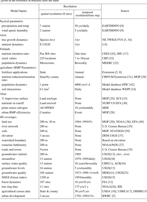
The scenarios were driven by changes in the Landuse map, the Sewers map, patterns of fertilizer application, amounts of atmospheric deposition, and location and number of dwelling units. Since the model is spatially explicit and dynamic, it generates a huge amount of output for each scenario run. We can only present a brief summary here in the form of spatially and temporally averaged values for a few key indica-tors. Table 1 is a summary of some of the model output from the different scenarios looking at nitrogen concen-tration in the Patuxent River as an indicator of water quality, changes in the hydrologic flow and changes in the net primary productivity of the landscape. Some selected additional results of the scenario runs are described briefly below.

Historical Scenarios

In this group of scenarios we attempted to recon-struct the historical development of the Patuxent water-shed, starting from the pre-European settlement condi-tions in 1650. The 1850, 1950 and 1972 maps (Fig. 1) were produced based on data from Buchanan et al. [3]. In 1650 the watershed was almost entirely forested, with very low atmospheric deposition of nitrogen, no fertilizers and no septic tank discharges. The rivers had very low nutrient concentrations. By 1850 the land-scape had been dramatically modified by European set-tlers. Almost all the forests were cleared and replaced with agriculture (Table 1). However fertilizers used at the time were mostly organic (manure, river mud, green manure, vegetable matter, ashes), the atmospheric dep-osition of nutrients was still negligible, and the popula-tion was low, producing little septic tank load.

After 1850, agricultural land use began shrinking and forests began regrowing. By 1950 the area of for-ests had almost doubled. At the same time, rapid urban-ization began, primarily along the Washington DC— Baltimore corridor. This affected the Patuxent water-shed both directly (through changes in land use from agriculture and forests to residential and commercial uses) and indirectly (through increased auto use in the larger region and increased atmospheric inputs of nutri-ents). This process continued until the 1970s, when reforestation hit it’s maximum. Since then, continued urbanization of the area has been affecting both agricul-tural and forested areas at approximately the same rate. The atmospheric emissions and fertilizer applications were assumed to grow steadily from the low pre-indus-trial levels to modern load levels. The growing popula-tion in the residential sectors was contributing to grow-ing discharges from septic tanks.

(‡) (b) (c) (d)

1 2 3 4 5

Table 1.

Some results of scenario runs for the Patuxent Model. The historical scenarios (1650–1972) are a reconstruction based on esti

mates done by USGS. The

“build-out” scenario was estimated based on the existing zoning maps and the average population densities for particular land use type

s. The buildout conditions represent the

“worst case” scenario. The ELUC scenarios (LUB1-4) are based on the model by N. Bockstael. Other scenarios are described in the

text. The table lists the land use

distribution for each scenario, followed by the nitrogen inputs from the atmosphere, fertilizers, decomposition, and septic tan

ks. Next are the average, max and min

Nitrogen in surface waters, and the max and min water levels in streams. W

max

is the total of the 10% of the flow that is maximal over a one year period. This represents

the peak flow. W

min

is the total of the 50% of flow that is minimal over a one year period. This is an indicator of the baseflow. N

gw.c

—is the average concentration on

N in the ground water. Since ground water is a fairly slow variable in the model and the model had only 1 year of relaxation ti

me in the experiments performed, this

variable probably does not adapt fast enough to track the changes assumed under the different scenarios. Total NPP (kg/m

2/yr) presents the average across the whole

watershed of plant productivity. It reflects the approximate proportion of forested and agricultural land use types, which have

a larger NPP than residential land uses.

See text for additional details Scenario

Ç

Land use types, number of cells

Ixnput of N, kg/ha/year

N concentrations in surface

waters, mg/l

504 VOINOV et al. 1990 vs. 1997 vs. Buildout

Comparison between the 1990 and 1997 model out-put shows that there was a considerable decline in the numbers of forested and agricultural cells, which was due to the increase in residential and urban areas. Accordingly, fertilizers contributed less to the total nitrogen load for the watershed, whereas the amount of nitrogen from septic tanks increased (Table 1). These load totals also demonstrate the relative importance of different sources of nitrogen on the watershed. Under existing agricultural practices the role of fertilizers remains fairly high. Atmospheric deposition contrib-utes unexpectedly high proportions of the nitrogen load. The role of septic tanks may seem minor, however it should be remembered that the fate of septic nitrogen is quite different from the pathways of fertilizer and atmospheric nitrogen. Under existing design of septic drainage fields, the septic discharge is channeled directly to groundwater storage almost entirely avoid-ing the root zone and nutrient uptake by terrestrial plants.

From 1990 to 1997 most of the land use change in the model occurred by replacing forested with residen-tial land use types. As a result we do not observe any substantial decrease in water quality in the Patuxent River (Table 1). The changes in hydrologic parameters that are associated with the substitution of residential areas for forested and agricultural ones result in some-what more variability in the flow pattern, however this difference is not very large. Apparently during this time period the residential land use is still less damaging than the agricultural one and the loss in environmental quality that is associated with a transfer from forested to residential conditions is compensated by a net gain in a similar transfer from agricultural to residential use.

These trends are reversed when we move on to the buildout (BO) conditions in the model. At some point a threshold is passed after which most of the develop-ment occurs due to deforestation and the effect of resi-dential and urban use becomes quite detrimental for the water quality and quantity in the watershed. The base-flow (represented by the 50% minimal base-flow values) decreases to almost half of the pre-development 1650 conditions, the peak flows become very high because of the overall increase of impervious surfaces. Accord-ingly the nitrogen content in the river water grows quite considerably.

Best Management Practices (BMPs)

The next scenario attempts to mimic the possible effects of BMPs. Government concerns are primarily aimed at nutrient reduction through non-point source control and growth management (MOP 1993) [28] and have the broader goal of improving the groundwater, river and estuarine water quality for drinking water and habitat uses. Non-point source control methods under study include: stream buffers, adoption of agricultural

and urban Best Management Practices (BMPs), and forest and wetland conservation. Urban BMPs or stormwater management, involve both new develop-ment and retrofitting older developdevelop-ments. Growth man-agement includes programs to cluster development, protect sensitive areas, and carefully plan sewer exten-sions. Clustered development has been proposed and promoted in Maryland as a method to reduce nonpoint sources and preserve undeveloped land.

At this time we have limited our consideration of BMPs to reduction of fertilizer application. Crop rota-tion has been assumed previously as a standard farming practice in the area. In addition to that we assessed the potential for nutrient reduction in the Patuxent from reductions achieved by farmers in the basin who have adopted farm nutrient management plans. The Mary-land Nutrient Management Program (NMP) enlists farmers who are willing to create and implement nutri-ent managemnutri-ent plans which use a variety of tech-niques to lower application rates including: nutrient crediting with and without soil testing, setting realistic yield goals, and manure testing and storage. The big-gest gains for farms without animal operations tended to come from adjusting yield goals (Patricia Steinhil-ber, Coordinator of the NMP, pers comm., 1996). From this information, we created an expected nutrient

reduction of 10−15%, which is the typical reduction for

farms in the NMP (Tom Simpson, MDA, pers. comm., 1996). Another major source of fertilizer application reduction is accounting for atmospheric deposition in calculations of nutrient requirements. This has been promoted by some of the recent recommendations issued by MDA. As a result we get quite a considerable change in fertilizer loading and reduction of agricul-tural land use in the watershed becomes no longer ben-eficial for water quality in the river (Table 2).

ECONOMIC LAND USE CONVERSION (ELUC) MODEL SCENARIOS

Table 2. PLM Data. Unless otherwise noted, spatial and temporal resolution refer to the source data. Data source information is given in the reference in brackets after the table

Model Inputs

Resolution

Source spatial resolution (# sites) temporal

resolution/time step Physical parameters

precipitation and temp 7 station 50 yrs/daily EARTHINFO [9]

wind speed, humidity 2 station 5 yrs/daily EARTHINFO [9]

Forest

tree growth dynamics Species leve 1/yr NE TWIGS FVS [5, 34]

nutrient dynamics E US/20 1/yr [14]

Wetlands

nutrient retention rates Pax R/6 sites One time CEES [43], JHU [17]

stock values 225 locations 7 to 10/year CBP [32]

population dynamics Mesocosms Beweekly MEERC [22]

Agriculture (BMP Parameters)

fertilizer applications State Annual Extension [2, 8]

nutrient reduction/retention rates

State/by county Annual CBP/UM Extension [31], MOP [28] population dynamics 1 point 4000 yrs/1 d Model database EPIC [42]

soil interactions 0.1 km2 _{Daily Model database WEPP [24]}

Urban

% impervious surface Land use/type None MOP [25], SCS [33]

nutrients in runoff Land use/soil None NURP US EPA [30]

point source nitrogen All NPDES 10 yrs/monthly MDE

urban BMP efficiencies Counties Event MOP [28]

GIS coverages

land use 200 m; 30 m 1984–1994/5× MOP [20], NOAA [36], EPA [40]

river network 200 m None U.S. Census Bureau [35]

soils 200 m None MOP, STATSGO [29]

elevation 3 arcsec None DEM USGS [37]

watershed boundary 200 m None Based on elevation

estuarine bathimetry 200 m None NOAA/NOS [27]

roads and towns Vector None U.S. Census Bureau [35]

groundwater (initial) 200 m 1985 USGS[13], elev., river

streamflow 13 station 1979–1995/daily USGS[38]

surface water quality 13 station 10 years/beweekly CBP[11], ACB[16]

groundwater levels 16 station 5 yrs/monthly USGS[13]

groundwater quality 105 station 1973–1990 1×/well MDE[41], USGS[23]

NDGI (Green index) 1250 m 1993/monthly USGS[15]

forest dynamics 187 sites 10 yrs/10 yrs FIA [12]

tree ring data 11 sites 175 yrs/1 y NOAA[26], IEE

agricultural census data State & county 50 yrs/5 yrs USDA [10], USBS [4.7], DHMH [19]

506 VOINOV et al. changes do not bring us to the threshold conditions after

which the residential trends of development become especially damaging to the environmental conditions.

HYPOTHETICAL SCENARIOS

In the next group of scenarios we considered some more drastic changes in land use patterns. None of these are realistic, but they allow one to estimate the rel-ative contributions of major land use types to the cur-rent behavior of the system. They were also essential to evaluate the overall robustness of the model and esti-mate the ranges of change that the model could accom-modate. For example by comparing Scenarios (14) and (15) one can see that agricultural land uses currently play a larger role in the nutrient load received by the river than residential land uses, even under the BMPs. We get a considerable gain in water quality by transfer-ring all the agricultural land into residential. Contrary to expectations, cluster development (Scenario 17) did not turn out to be any better for river water quality than residential sprawl (18). Because of larger impervious areas associated with urban land use, the peak runoff dramatically increased in this scenario. This in turn increased the amount of nutrients washed off the catch-ment area. Cluster developcatch-ment would be beneficial only if it is accompanied by effective sewage and storm water management that will reduce runoff and provide sufficient retention volumes to channel water off the surface into the ground water storage. It should be noted however that in our definition of these scenarios we have only modified the land use maps in terms of the limited number of aggregated categories that we are distinguishing. The changes in the infrastructure (roads, communications, sewers, etc.) that should be associated with the cluster vs. sprawl development have not yet been taken into account.

Conversion of all currently forested areas into resi-dential (Scenario 16) was almost as bad as the Build Out scenario (7). However the crop rotation assumed in (16) decreased the amounts of fertilizers applied some-what and resulted in lower overall nitrogen concentra-tions. The septic load in this case was so large because the transition to residential land use was assumed to occur without the construction of sewage treatment plants. In the Build Out scenario most of the residential and urban dwellings were created in areas served by existing or projected sewers.

SUMMARY OF SCENARIO RESULTS One major result of the analysis performed thus far is that the model behaves well and produces plausible output under significant variations in forcing functions and land use patterns. It can therefore be instrumental for analysis and comparisons of very diverse environ-mental conditions that can be formulated as scenarios of change and further studied and refined as additional data and information are obtained. The real power of

the model comes from its ability to link spatial hydrol-ogy, nutrients, plant dynamics and economic behavior via land use change. The economic sub-model incorpo-rates zoning, land use regulations, and sewer and septic tank distribution to provide an integrated method for examining human response to regulatory change. The projections from the economic model of land use change based on proposed scenarios shows the proba-ble distribution of new development across the land-scape so that the spatial ecological aspects can be eval-uated in the ecological model. The model allows fairly site specific effects to be examined as well as regional impacts so that both local water quality and Chesa-peake Bay inputs can be considered.

The scenario analyses also demonstrated that the Patuxent watershed system is complex and its behavior is counterintuitive in many cases. For example, in the entirely forested watershed of 1650 the flow was very well buffered showing very moderated peaks and fairly high baseflow. The agricultural development that fol-lowed in the next century actually decreased both the peak flow and the baseflow, contrary to what one would expect, even though the decrease in the baseflow was much more significant than the decrease in the peaks. Apparently evapotranspiration rates for the kinds of crops currently included in the model were high enough to keep the peaks down. Comparing the effects of vari-ous land use change scenarios on the water quality in the river (Fig. 2) similarly shows that the connection between the nutrient loading to the watershed and the nutrient concentration in the river is complex and diffi-cult to anticipate or generalize. This merely confirms the need for a complex, spatially explicit simulation model of the type we have developed here.

Nevertheless, a few general patterns emerge from analysis of the scenario results, including:

As previously observed [2], the effects of tempo-rarily distributed loadings are less pronounced than event-based ones. For example, fertilizer applications that occur once or twice a year increase the average nutrient content and especially the maximum nutrient concentration quite significantly, whereas the effect of atmospheric deposition is much more obscure. The dif-ference in atmospheric loading between Scenarios (1) and (3) is almost 2 orders of magnitude, yet the nutrient response is only 5–6 times higher, even though loadings from other sources also increase. Similarly the effect of septic loadings that are occurring constantly is not so

large. The average N concentration is well correlated

(r = 0.87) with the total amount of nutrients loaded. The

effect of fertilizers is most pronounced among the

indi-vidual factors (r = 0.82), while the effect of other

sources is much less (septic r = 0.02; decomposition

r = 0.40; atmosphere r = 0.71). The fertilizer

applica-tion rate determines the maximum nutrient

concentra-tions (r = 0.76), with the total nutrient input also

play-ing an important role (r = 0.55). Even the groundwater

appli-cations (r = 0.64), however in this case the septic

load-ings are more important (r = 0.68), even a more

impor-tant one than the total N loading (r = 0.52).

The hydrologic response is quite strongly driven by the land use patterns. The peak flow (max 10% of flow)

is determined by the degree of urbanization (r = 0.61).

The baseflow (min 50% of flow) is very much related to

the number of forested cells (r = 0.78), but in both cases

there are obviously other factors involved.

We used the net primary productivity (NPP), excluding agriculture and urban areas, as an indicator of ecosystem health and ecosystem services. The NPP is primarily provided by forested areas in the water-shed. Different land use patterns result in quite signifi-cant variations in NPP, both in the temporal (Fig. 3) and in the spatial domains. The predevelopment 1650 ditions produce the largest NPP, under Build Out con-ditions NPP is the lowest. Interestingly, there are cer-tain areas that currently produce higher NPP than in 1650. This is because of increased nutrient availability due to atmospheric deposition and fertilizer applica-tions in adjacent agricultural areas.

CONCLUSIONS

Linked ecological economic models like the PLM are potentially important tools for addressing issues of land use change at the regional watershed scale. The model integrates our current understanding of ecologi-cal and economic processes at the site and landscape scales to give estimates of the effects of spatially explicit land use or land management changes. The

model also highlights areas where knowledge is lacking and where further research should be targeted. Specifi-cally, the PLM model represents advances in the fol-lowing areas:

The model links topography, hydrology, nutrient dynamics, and vegetation dynamics at a fairly high temporal (1 day) and spatial (200 m) resolution with land use patterns and the longer term dynamics of land use change. As far as we know, it is the most advanced model of its type for application at the regional water-shed scale.

0 100 200 300 400 0 20 40 60 80 100

N, mg/l

1 2 3

1 2 3 4

1 2 3 4 5 6 7 8 9 10 11 12 13 14 15 16 17 18

Scenarios

(‡)

(b)

Fig. 2. Nitrogen loading and concentration of nitrogen in the Patuxent river under different scenarios of land use.

0 0.01 0.02 0.03 0.04

1 91 181 271 361 451 541 631 721 Day NPP, kg/(m2day)

1 2 3 4 5

508 VOINOV et al. The model allows the impacts of the spatial pattern

of land use on a large range of ecological indicators to be explicitly assessed, providing decision makers and the public with information about the consequences of specific land use patterns.

The model has been extensively calibrated over sev-eral time and space scales, a difficult and often ignored operation for models at this scale and complexity. New methods based on multi-criteria decision models were developed for this purpose.

The model operates at several scales simulta-neously, including the site (or unit model) scale and the landscape scale, which integrates all the unit models.

The model is process-based, with processes chang-ing in dominance over time. This allows better under-standing of the underlying phenomenon occurring on landscapes and therefore more detailed predictions of the possible results of changing land uses and policies. While the model is formulated deterministically, extensive sensitivity analysis, allows us to understand its complex dynamics without resorting to multiple sto-chastic replications. In the full spatial mode, when cells change from one land use type to another, a bifurcation threshold is simulated, and all the parameters in the cell change to those of the new land use type.

The high data requirements and computational com-plexities for this type of model mean that development and implementation are relatively slow and expensive. However, for many of the questions being asked this complexity is necessary. We have tried to find a balance between a simple, general model, which minimizes complexity and one that provides enough process-ori-ented, spatially and temporally explicit information to be useful for management purposes.

Spatial data is becoming increasingly available for these types of analyses and our modeling framework is able to effectively use this data to model and manage the landscape. One can also use the model to estimate the value of specific data collection investments for a particular model, watershed, and set of goals.

Because of the high complexity and large uncertain-ties in parameters and processes, any numerical esti-mates generated are intended to be used with caution. The high data requirements and computational com-plexities impede model development and implementa-tion.

The goal of a given study ultimately justifies the application of a certain modeling approach. In the case of large watersheds with complex and diverse ecosys-tem dynamics and extensive data requirements, the model inevitably needs fine tuning to the peculiarities of local ecological processes and the specifics of avail-able information. With models of such computational burden we want to avoid all possible redundancies. Therefore, the approach based on modeling systems and constructors that offer the flexibility of building models from existing functional blocks, libraries of

modules, functions and processes [21, 39], seems to be more appropriate for watershed modeling.

The Modular Modeling Language that we use offers the promise that models of varying degrees of detail can be archived, and made available for interchange during new model development. Then, for implementing a model for a particular area, modules can be selected based on the relative importance of local processes and high detail can be used where needed and otherwise avoided. The flexibility of rescaling the model spatially, temporally and structurally, allows us to build a hierar-chical array of models varying in their resolution and complexity to suit the needs of particular studies and challenges, from local up to global ones. With each aggregation level and scheme chosen, we can view the output within the framework of other hierarchical levels and keep track of what we gain and what we lose.

“SMART GROWTH”

The PLM model can be used to analyze the impacts of specific development and/or regulatory policies. A couple of our current scenarios deal directly with these issues. For example, the policy sometimes referred to as “smart growth” has achieved some currency, and has been advocated by several states, including Wisconsin and Maryland. “Smart” in this context is usually taken to mean “clustered” rather than “sprawled” develop-ment of new residential and commercial activities on the landscape. Scenarios 17 (residential clustering) and 18 (residential sprawl) look at the effects of a hypothet-ical clustering or sprawling of the existing residential land uses. The clustering scenario converts all current low density residential land uses in the watershed to urban around three major centers, leaving everything else the same as the base case scenario. The sprawl sce-nario converts all current high density urban into resi-dential, randomly spread around the watershed. Table 2 shows some of the characteristics and impacts of these scenarios.

Compared to the 1997 baseline, the clustered

sce-nario had 276 km2 _{of urban, compared to 92 km}2_{, and}

0 km2 _{of residential compared to 311 km}2_{, while the}

sprawled scenario had 652 km2 _{of residential and 0 km}2

of urban. Forest and agricultural areas and nutrient inputs were adjusted accordingly. For example, the

clustered scenario had an average of 17 kg/ha/yr of N

input from septic tanks, compared to 18 kg/ha/yr for the base case and 27 kg/ha/yr for the sprawled scenario.

The sprawled scenario also had average fertilizer N

input (101 kg/ha/yr) larger than both the clustered sce-nario (89 kg/ha/yr) and the base case scesce-nario (100 kg/ha/yr) due to additional inputs from more lawns.

The clustered scenario is better in terms of N in

streams, with lower values of the average (10.5 mg/l)

and W_max (30.06 mg/l) than the base case (12.37 and

Wmin (1.33 and 1.37 mg/l). The sprawled scenario is much worse with 13.5, 45.14, and 3.55 mg/l, respec-tively. The clustered scenario is a bit ambiguous in terms of hydrology compared to the base case, with

higher Wmax and Wmin. This is due to the increased storm

water runoff from urban areas, vs. dispersed residential. This effect could be ameliorated with adequate urban storm water management—which was not assumed to be present in the current scenario run. The sprawled

scenario had a lower Wmax and about the same Wmin

compared to the base case, due to the replacement of agricultural land with low density urban. Ground water

N was lower in the clustered and higher in the sprawled

scenario than the base case. Finally, NPP was

signifi-cantly higher in the clustered scenario (1.868 kg/m2_/yr)

than the base case (1.627 kg/m2_{/yr) and lower in the}

sprawled scenario (1.271 kg/m2_{/yr). Higher NPP}

corre-lates with a higher production of ecosystem services (see above) and a higher quality of life.

MODELING AND DECISION MAKING Humans interact with the model in two distinct, but complementary ways. First, stakeholders were involved in developing the model and can use the model to address policy and management issues. In this mode human decision-making is outside the model, but inter-acts with the model iteratively. The model is affected by decisions stakeholders make via changes the modelers make in response to the stakeholder’s input, and new scenarios that are run in response to their requests.

In the second mode, human decision-making is internalized in the model. Only a few models have attempted to fully integrate ecological systems dynam-ics and endogenous human decision making (cf. [6]), and none of these have been spatially explicit. In this mode, one tries to model the human agent’s responses to the changing conditions in each cell, and the changes in built, human, and social capital. So far in the PLM, modeling of human decision-making has been limited to the economic land use conversion model discussed earlier. We are currently adding local socioeconomic dynamics to the unit model to further internalize human decision-making.

These two modes are complementary because observing how people make decisions interacting with the version of the model that does not include human decision-making can help us understand and calibrate the version of the model that does include human deci-sion-making internally.

We have been quite successful so far in using the model in mode one at several scales. Most land use pol-icy decisions in Maryland are made at the county level, and we have been interacting with several counties (in particular Calvert County) using the model to address land use policy decisions. For example, we performed a detailed case study of the Hunting Creek subwater-shed for the Calvert County Planning Commission to

address questions of land use impacts on stream water quality (see http://giee.uvm.edu/PLM for details) [44]. At the federal level, EPA and other environmental man-agement agencies, are, as we said at the beginning of this article, getting much more involved in watershed and landscape level analysis and policy making. For these agencies it is not so much the specific results for the Patuxent watershed that are of most interest, but the general technique and the general results that may be applicable to all watersheds. The landscape modeling techniques we have developed are certainly applicable to any watershed, and many of the scenarios we reported in this paper are relevant to some of the gen-eral policy questions that EPA and other environmental management agencies are addressing. These include the impacts of buildout (scenario 7), agricultural best management practices (scenario 8), the overall impacts of agriculture (scenario 14) and residential develop-ment (scenario 15), and the effects of sprawl and clus-tering (scenarios 17 and 18, see above). Models like the PLM are essential tools to improve our ability to make informed regulatory policy decisions at the watershed and landscape scales.

ACKNOWLEDGMENTS

Initial funding for this research came from the U.S. EPA Office of Policy, Planning and Evaluation (Coop. Agreement No. CR821925010). Funding has been provided by the U.S. EPA/NSF Water and Water-sheds Program through the US EPA Office of Research and Development (grant no. R82-4766-010).

Our sincere thanks go to those researchers who shared their data and insights with us, including eco-nomic modelers: Nancy Bockstael, Jacqueline Geoghe-gan, Elena Irwin, Kathleen Bell, and Ivar Strand and other researchers including: Walter Boynton, Jim Hagy, Robert Gardner, Rich Hall, Debbie Weller, Joe Tassone, Joe Bachman, Randolph McFarland, and many others at the Maryland Dept. of Natural Resources, Maryland Dept. of the Environment and the University of Mary-land Center for Environmental Studies. Special thanks go to Carl Fitz and Lisa Wainger who were working on initial stages of the project.

REFERENCES

1. Baltimore–Washington Regional Collaboratory, 200 Years of Spatial Data, UMBS, NASA, USGS. http://research.umbc.edu/ ~tbenja1/bwhp/main.html 2. Bandel, V.A. and Heger, E.A., MASCAP–Maryland’s

Agronomic Soil Capability Assessment Program, Uni-versity of Maryland Cooperative Extension Service and Department of Agronomy in cooperation with USDA Soil Conservation Service: College Park, MD. Mary-land: MD, 1994.

510 VOINOV et al. 4. Bureau of the Census, 1987 Census of Agriculture,

vol. 1, Geographic Area Series, no. 20, Maryland: State and County Data, US Department of Commerce: Wash-ington, DC, 1989.

5. Bush, R.R., Northeastern TWIGS Variant of the Forest Vegetation Simulator, Forest Management Service Cen-ter, 1995.

6. Carpenter, S., Brock, W., and Hanson, P., Ecological and Social Dynamics in Simple Models of Ecosystem Man-agement, Conservation Ecology, 1999, vol. 3, no. 4. 7. Census of Agriculture: 1982, 1987, 1992, Government

Information Sharing Project: Oregon State University– Information service. http://govinfo.kerr.orst.edu/ag-stateis.html

8. Coale, F., Fertilizer application rate and timing, Coop-erative Extension Service, College Park, MD, 1995. 9. EARTHINFO, I., NCDC Summary of the Day. East

1993., EARTHINFO, Inc.: Boulder, CO.

10. Economic Research Service, U., ERS Databases., http://www.econ.ag.gov/Prodsrvs/dataprod.htm

11. EPA Chesapeake Bay Program, Water Quality Monitoring. Data Sets and Documentation., http:// www.epa.gov/docs/r3chespk/cbp_home/infobase/wqual/ wqgate.htm

12. Hansen M.H., Frieswyk T., Glover J. F., Kelly J. F. The Eastwide Forest Inventory and Analysis Data Base: Users Manual, http://www.srsfia.usfs.msstate.edu/ ewman.htm

13. James, R.W.J., Horlein, J.F., Strain, B.F., and Smigaj, M.J., Water Resources Data, Maryland: and Delaware. Water year, 1990.

14. Johnson, D.W. and Lindberg, S.E., Atmospheric Deposi-tion and Forest Nutrient Cycling: a Synthesis of the Inte-grated Forest Study, New York: Springer, 1992.

15. Jones, J., Normalized-Difference Vegetation Index, Research & Applications Group. Reston: USGS, 1996. 16. Judd, M., Citizen Monitoring Data, Alliance for the

Chesapeake Bay, 1996.

17. Kahn, H. and Brush, G.S., Nutrient and Metal Accumu-lation in a Freshwater Tidal Marsh, Estuaries, 1994, vol. 17, no. 2, pp. 345–360.

18. Krysanova, V., Simulation Modelling of the Coastal Waters Pollution from Agricultural Watershed, Ecol. Modell., 1989, vol. 49, pp. 7–29.

19. Maryland: Department of Health and Mental Hygiene, Description of the Patuxent Watershed Nonpoint Source Water Quality Monitoring and Modeling Program Data Base and Data Base Management System, 1986, MDE, Office of Environmental Programs, Water Management Administration, Division of Modeling and Analysis. 20. Maryland Office of Planning. Maryland State Data

Cen-ter. http://www.inform.umd.edu/UMS + State/MD_Resources/MSDC/

21. Maxwell, T. and Costanza, R., A Language for Modular Spatio-Temporal Simulation, Ecol. modelling, 1997, vol. 103, no. 2, pp. 105–114.

22. Multiscale Experimental Ecosystem Research Center— MEERC. Welcome to the MEERC World Wide Web (W3) Server. http://kabir.cbl.cees.edu/Welcome.html

23. McFarland, E.R., Relation of Land Use To Nitrogen Concentration in Ground Water in the Patuxent River Basin, Maryland, 1995.

24. National Soil Erosion Laboratory. Water Erosion Pre-diction Project (WEPP). http://soils.ecn.purdue.edu/ ~wepphtml/wepp/wepptut/ahtml/avi/welcome.au 25. Natural Soil Groups of Maryland Technical Report,

Maryland Office of Planning. MD Dept. of State Plan-ning. December, 1973.

26. NOAA Paleoclimatology Program, Tree Ring Data. http://www.ngdc.noaa.gov.paleotreering.html

27. NOAA/National Ocean Service, MapFinder. Preview Demonstration of August 1997 Offering. http://mapin-dex.nos.noaa.gov/

28. Nonpoint Source Assessment and Accounting System, Maryland: Office of Planning and Maryland Dept. of Environment, 1993.

29. NRCS USDA, State Soil Geographic (STATSGO) Data Base. http://www.ncg.nrcs.usda.gov/statsgo.html 30. Results of the Nationwide Urban Runoff Program, U.S.

Environmental Protection Agency, Water Planning Divi-sion, Washington, DC: 1983.

31. Steinhilber, P., FY 95 New Plan Fertilizer N, P205, and K20 Reductions for Selected Groups, Nutrient Manage-ment Program, 1995.

32. The Biological Data and Information Page, EPA Chesa-peake Bay Program. http://www.epa.gov/docs/r3chespk/ cbp_home/infobase/lr/lrsctop.htm

33. The Forest Vegetation Simulator (FVS) and Insect and Pathogen Models., USDA Forest Service. http://162.79.41.7/fhtet/background.html

34. Urban Hydrology for Small Watersheds, USDA Soil Conservation Service, Engineering Division. 1975. 35. U.S.Census Bureau, TIGER: The Coast to Coast Digital

Map Database, http://www.census.gov/geo/www/tiger/ 36. USDC NOAA Coastal Service Center, C-CAP. Coastal

Change Analysis Program, http://www.csc.noaa.gov/ ccap/

37. USGS, USGS Digital Elevation Model Data, http://edcwww.cr.usgs.gov/glis/hyper/guide/usgs_dem 38. USGS, Maryland Surface-Water Data Retrieval,

http://h2o.usgs.gov/swr/MD/

39. Voinov, A. and Akhremenkov, A., Simulation Modeling System for Aquatic Bodies, Ecol. Modeling, 1990, vol. 52, pp. 181–205.

40. Vogelmann, J., MRLC Landuse Coverages for 1992–93, EROS Data Center, 1996

41. Wilde, F.D., Geochemistry and Factors Affecting Ground-Water Quality at Three Storm-Water-Manage-ment Sites, Maryland: DepartStorm-Water-Manage-ment of Natural Resources Maryland Geological Survey in cooperation with USGS, Maryland Department of the Environment and the Gov-ernor’s Commission on Chesapeake Bay Initiatives, 1994. 42. Williams, J.R, Dyke, P.T, and Jones, C.A, in Analysis of

Ecological Systems: State-of-the-Art in Ecological Mod-eling, Laurenroth, W.K., Ed., Amsterdam: Elsevier, 1983, pp. 553–572.

43. Zelenke, J.L. and Cornwell, J.C., Nutrient Retention in the Patuxent River Marshes, Horn Point Environmental Laboratory, UMD, Cambridge: MD, 1996.