Improvement of effort estimation accuracy in
software projects using a feature selection approach
Zahra Shahpar1, Vahid Khatibi2, Asma Tanavar3, Rahil Sarikhani4
Received (2016-06-06) Accepted (2016-12-06)
Abstract — In recent years, utilization of feature selection techniques has become an essential requirement for processing and model construction in different scientific areas. In the field of software project effort estimation, the need to apply dimensionality reduction and feature selection methods has become an inevitable demand. The high volumes of data, costs, and time necessary for gathering data, and also the complexity of the models used for effort estimation are all reasons to use the methods mentioned. Therefore, in this article, a genetic algorithm has been used for feature selection in the field of software project effort estimation. This technique has been tested on well-known datasets. Implementation results indicate that the resulting subset, compared to the original dataset, has produced better outcomes in terms of effort estimation accuracy. This article showed that genetic algorithms are ideal methods for selecting a subset of features and improving effort estimation accuracy .
Index Terms — dimensionality reduction, feature selection, genetic algorithm, software effort estimation.
I. INTRODUCTION
O
ne of the important and effective stages ina software engineering process which can play an important role in the success or failure of
the project is effort and cost estimation [1]. The two phrases cost estimation and effort estimation
are usually equivalently used in software
engineering and project management surveys [2]. Accurate effort estimation for resource allocation and project planning is of great importance. Underestimating a software project effort causes
delays in project scheduling, increases costs, and
eventually leads to the projects’ failure. On the other hand, overestimation of a project effort in effectively utilizing software resources has its own side effects [1].
Accurate estimation of a software project
effort is a difficult task considering that multiple parameters are used in software project effort estimation. The data sets used are mostly
multi-dimensional, which despite creating certain opportunities, also create many computational
challenges. One of the existing problems in
this regard is that not all features are critical
for finding the hidden knowledge amongst the
important data, and in many cases, some of the
candidate features are unrelated and redundant.
In addition, the gathering of these data is time
consuming and highly costly. These unnecessary
features dramatically reduce the algorithms
learning speed and accuracy. Moreover, recent
surveys have shown that data quality and the
fitness of the datasets utilized in effort estimation
techniques are key factors for achieving better
results. Additionally, through selecting subsets
from these features, we are able to reduce
the model estimation complexity. Therefore,
1- Department of Computer Engineering, Kerman Branch, Islamic Azad University, Kerman, Iran.(zahrashahpar@ yahoo.com)
2- Faculty Member of Islamic Azad University, Kerman Branch, Iran.
selecting related and necessary features is of fundamental importance for increasing model
efficiency [3, 4].
Therefore, this article attempts to apply a feature selection method for improving accuracy
and efficiency of effort estimation. We will present our proposed method for examining datasets
in section 2, after reviewing the researches
accomplished in the field of effort estimation and
feature selection, and in the 3rd section, we will
examine the methods evaluation measures, and in the 4th and final sections of the article, we will analyze the concluded results.
II. REVIEW OF LITERATURE
In this section, we will review background studies with respect to two approaches; software
project effort estimation and feature selection: The initial idea of effort estimation dates back to the 1950s. In 1965, with increases in software
projects and demand for high quality software,
regression techniques were deployed for effort estimation [5]. During 1970, the COCOMO model was formulated by Barry W.Boehm and C.Bats. During the 1980’s, many developments were made on effort estimation models and
methods including the changes applied by
Boehm et al on COCOMO, which resulted in the new model, COCOMO II [6]. Therefore, it can be
said that during the last years, many studies were
made in the field of effort estimation leading to increases in effort estimation accuracy including the following cases:
Filomena Ferrucci et al [7] used genetic programing for effort estimation and result analysis. They indicated that genetic
programming, in comparison with other methods,
increases estimation accuracy. Mandeep Singh et al [8] presented a practical model for early estimation of software development. After data analysis, they calculated the influence of different parameters on productivity. Mohammad Azzeh et al [9] used an artificial bee colony algorithm
for determining the appropriate number and
factor of each feature for software project effort estimation. They evaluated this method on 8 promising datasets. Rahul Premraj et al [10]
presented a model for cost estimation using
homogenous data.
On the other hand, feature selection has been
examined in different perspectives at the hands
of various authors. It can be said that the purpose
of feature selection is to select a certain subset
of features in order to increase effort estimation accuracy. In other words, reduction in structure size will occur without any significant reductions
in estimation accuracy, which is obtained through
utilizing the features presented [3].
Different feature selection methods can be categorized into various sets according to search methods. In some methods, the whole space
possible is searched completely whereas in other methods, the search space may become smaller
with a trade-off of losing a little efficiency [3]. Each of these methods can be categorized into different fields according to their application. In
the following, some of the methods used in cost
and effort estimation are mentioned.
Efi Papatheocharous et al. [4] examined four
feature selection methods including stepwise
regression Garson’s algorithm on artificial neural
networks (ANN), forward selection, backward elimination, and genetic algorithm using a ridge regression and last squares technique on two
datasets; Desharnais and ISBSG.
Karagiannopoulos et al. [11] compared five wrapper feature selection methods using regression algorithms. The wrapper approach is known as the black box method in which a scale
function is used to evaluate the appropriateness
of feature subsets. Methods used in this article
include Forward Selection (FS), Backward Selection (BS), the Best First forward selection (BFFS), the Best First Backward Selection
(BFBS), and Genetic Search Selection (GS). The regression algorithms used are: Regression Trees,
Regression Rules, Instance-Based Learning
Algorithms, and Support Vector Machines. Also, in order to execute the method and analyze the
results, 12 uci datasets have been used in this
article.
III. METHODOLOGY
As previously mentioned, this research was
performed with the purpose of increasing effort estimation accuracy using feature selection. In
this research, a genetic algorithm has been used for
feature selection. So far only statistical techniques,
regression, and evolutionary algorithms have
been used. The bee colony algorithm has been used in numerous effort estimation scenarios for different software projects [5-10]. Also, different
different datasets. However, genetic algorithms have not been amongst these methods [3-4-11].
Thus, this study focuses on proposing a genetic algorithm for feature selection, which will be
explained further in the next sections. Before
applying this genetic algorithm on datasets, in order to prevent problems related to the huge
differences of magnitudes, calculations, and the overflow of variables, the data have been normalized such that all independent variables in
the used data sets have been mapped to a number
within the interval of [0-1]. Then, the data have been categorized into testing and learning sets
using a 3-fold standard method and the genetic algorithm has been implemented on the learning
data. The working procedure is shown in figure 1. Therefore, after examining the evaluation
method and the proposed performance evaluation
method, we will describe and examine the genetic
algorithm, cost function of the genetic algorithm,
and the utilized data sets.
1.Evaluation Method
A 3-fold standard method has been used for
result evaluation. In this method, the target dataset is first randomly divided into 3 approximately
equal parts and each time one of these three parts is used as the testing data and the 2/3 left is used as the learning data for genetic algorithm cost
function optimizations. This procedure is repeated 30 times and then the results are examined.
2. Operational Parameters
Many evaluation criteria have been defined and utilized in effort and cost estimation techniques.
The four very common evaluation criteria used
in studies are MRE which is the effort estimation difference error rate by the algorithm using real efforts, mean MRE (MMRE) which is the
mean estimation error rate for all target samples
(learning or testing), median MRE (MDMRE) or
the median error rate of the amount determined
by the algorithm using real effort samples, and finally PRED(x) which is the percentage of
samples which had an error rate of less than or
equal to x. These four parameters are calculated as follows [5, 12]:
rt ActualEffo
ffort EstimatedE rt
ActualEffo
MRE = − (1)
In which Actual Effort is the amount of effort
of the real target project within the dataset and
Estimated Effort is the estimation effort evaluated by the algorithm [5].
∑
=
− = n
i ActualEffort
ffort EstimatedE rt
ActualEffo n
MMRE 1
.
1
(2)
In which n denotes the number of projects
evaluated. Lower MMRE indicates lower
estimation error of the algorithm, which implies
better accuracy [12].
) (MRE median
MDMRE= (3)
n k X
PRED( )= (4)
In which X is the target difference which in most studies is 0.25, K denotes the number of samples for which the difference of effort
estimated by the algorithm along with the real
effort are less than or equal to X, n is the total number of samples being evaluated [5].
3. Genetic Algorithm
The JACET algorithm was introduced by John
Holland (1967). This method later became very popular with the help of Goldberg (1989). In this
method, based on the gradual evolution theory and other fundamental ideas of Darwin, an initial set of target parameters is randomly produced for a constant number of samples namely the initial
population. Then, the simulation program is executed and the number indicating the standard
deviation or the practice of that information set
is ascribed to the given population (fitness). This
procedure is repeated for each and every member
produced. Then, by calling the genetic algorithm
operators including crossover and mutation,
the next generation selection is formed and
the routine is continued until the convergence
criterion is met [13].
In this study, using a genetic algorithm,
a random population with a constant size of
50 members from the candidate features is
produced. The feature set presented or namely
the chromosomes are shown as a binary string
with length n in which a zero or one at location
i of the string shows the presence or absence of
feature i in the feature set selected. n is the total number of features available. In each iteration,
current population is determined using a cost
function which is explained later and the optimal members are selected as the next generation population. New chromosomes are created from
the previous chromosomes using the crossover
and the mutation procedures. In this study, three
methods of single point crossover, double point crossover, and uniform crossover are used and a
rate of 0.08 is selected for the mutation procedure using a swap method with a rate of 0.3, and the
mutation probability for each gene is considered
as 0.02. For the selection, the Roulette Wheel method with a selection pressure of 8 is used. This
routine is iterated until it reaches the intended number of iterations and the optimal amount for
the cost function.
Figure 1. Study workflow and feature selection
4. Cost Function
The cost function used in the genetic algorithm of this study is a double target cost function in
which by reducing the amount of MMRE, the
minimal number of possible features is selected
from the dataset. In the following equation, β is
an independent positive number indicating the cost of adding a feature with which we can create balance between the two scales nf (number of
selected features) and MMRE (mean estimation error rate for all target samples).
) * 1 ( nf MMRE
MINZ= +β (5)
In order to calculate the MMRE, a hybrid
linear regression and a decision tree has been
used. Regression analysis is a statistical method
for estimating the relation between variables creating an opportunity for predicting the impact of one variable on multiple variables and giving a better understanding of a variable change status
at the change time of each independent variable.
The regression model calculates Y as a function
of X and β in which β is the unknown parameter,
X is the independent variable, and Y is the
dependent variable [8].
) , (X β
Y = (6)
The decision tree is a flow chart with a tree
structure in which each inner node performs
a test on one of hybrid features. Each branch
shows an output of the test and each leaf node indicates the label or estimated amount for that
sample. The strongest node of a tree is the root [14]. In this study, we made use of classification and regression tree (cart) algorithms.
5. Datasets
The datasets used in this study are Maxwell, Cocomo81, and Desharnais. The reason for
choosing these three datasets is that these sets contain relatively new data on a large number of software projects from the largest banks in the world are perhaps some of the most common
datasets used in effort estimation studies. Thus,
these datasets were chosen in order to compare
the concluding results with other studies [5-15-16]. The datasets will be explained in further detail.
The Maxwell dataset includes relatively new data in 62 fields of software projects from the
largest world banks in Finland in which each
project describes 26 features. This data set has
25 independent variables with various software
The Cocomo81 dataset includes 63 software projects such as commercial, scientific, systematic, on-time, and support projects. It has
16 independent variables which are measured using product, project, computer, and personal
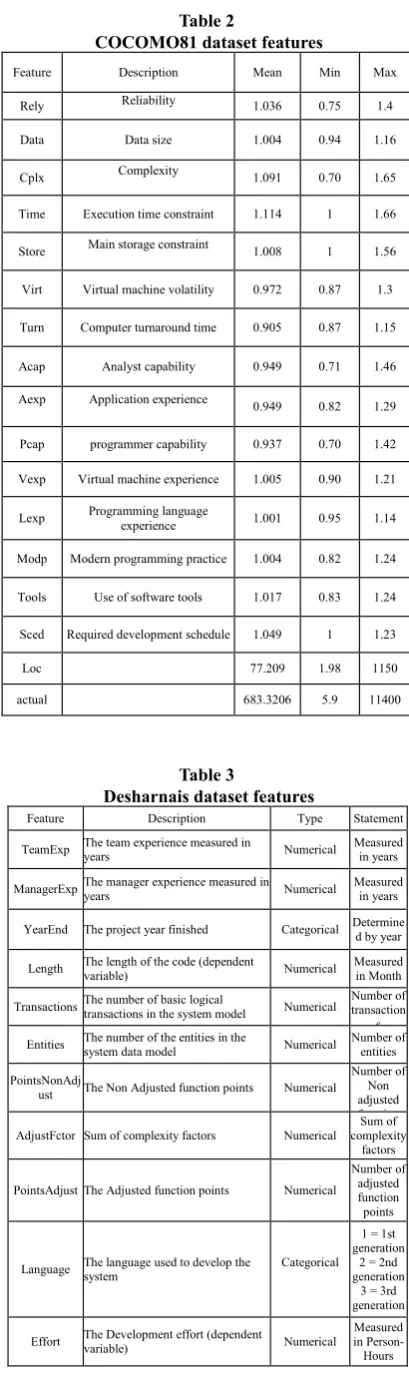
attributes. The dependent variable is the software development effort measured using each individual’s hours [15]. Statistical information related to the Cocomo81 dataset are presented in table 2.
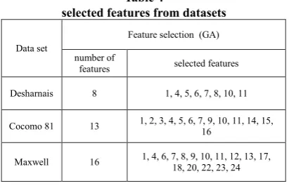
The Desharnais dataset is one of the most
common datasets in effort estimation. This dataset includes 81 software project samples in
which four samples include faulty data; thus, only
77 samples have been considered. In this dataset,
each sample is described using 11 features, 10 of which are independent, and only one feature
is dependent. In this study, the dependent effort variable estimation has been used using each individual’s hours [16]. Explanations
and information about the Desharnais dataset
variables are presented in table 3.
IV. RESULTS
In this section, the outcomes of performing this study according to the method proposed
in previous sections will be examined. The proposed method is executed and evaluated on MATLAB software using the three datasets Maxwell, COCOMO81, and Desharnais. As
mentioned before, feature selection is done using
a binary genetic algorithm, and for examining the
evaluation criterion, a hybrid linear regression method and a decision tree along with a tree
regression algorithm has been used. Results of
hybrid linear regression analysis before and after
feature selection are presented in figure 2 which shows a reduction in parameters of MMRE, MdMRE, and STD and an increase in PRED for
the three given datasets after applying genetic
algorithm and feature selection. 8, 13, and 16
features have been selected from the Desharnais
dataset with 10 features, COCOMO81 dataset with 16 features, and Maxwell data with 25 features, respectively.
Table 1
Maxwell dataset features
Feature Description Mean Std Dev Min Max
Time Time 5.58 2.13 1 9 App Application type 2.35 0.99 1 5
Har Hardware platform 2.61 1 1 5 Dba Database 1.03 0.44 0 4 Ifc User interface 1.94 0.25 1 2 Source Where developed 1.87 0.34 1 2 Telonuse Telon use 2.55 1.02 1 4
Nlan
Number of different development
languages
used 0.24 0.43 0 1 T01 participationCustomer 3.05 1 1 5
T02
Development environment
adequacy 3.05 0.71 1 5 T03 Staff availability 3.03 0.89 2 5 T04 Standards use 3.19 0.70 2 5 T05 Methods use 3.05 0.71 1 5 T06 Tools use 2.90 0.69 1 4
T07 Software’s logicalcomplexity 3.24 0.90 1 5
T08 Requirementsvolatility 3.81 0.96 2 5 T09 requirementsQuality 4.06 0.74 2 5 T10 requirementsEfficiency 3.61 0.89 2 5 T11 requirementsInstallation 3.42 0.98 2 5 T12 Staff analysis skills 3.82 0.69 2 5 T13 Staff applicationknowledge 3.06 0.96 1 5 T14 Staff tool skills 3.26 1.01 1 5 T15 Staff team skills 3.34 0.75 1 5 Duration Duration 17.21 10.65 4 54
Table 2
COCOMO81 dataset features
Feature Description Mean Min Max
Rely Reliability 1.036 0.75 1.4
Data Data size 1.004 0.94 1.16 Cplx Complexity 1.091 0.70 1.65
Time Execution time constraint 1.114 1 1.66
Store Main storage constraint 1.008 1 1.56
Virt Virtual machine volatility 0.972 0.87 1.3
Turn Computer turnaround time 0.905 0.87 1.15
Acap Analyst capability 0.949 0.71 1.46 Aexp Application experience 0.949 0.82 1.29 Pcap programmer capability 0.937 0.70 1.42 Vexp Virtual machine experience 1.005 0.90 1.21 Lexp Programming language experience 1.001 0.95 1.14 Modp Modern programming practice 1.004 0.82 1.24
Tools Use of software tools 1.017 0.83 1.24
Sced Required development schedule 1.049 1 1.23
Loc 77.209 1.98 1150 actual 683.3206 5.9 11400
Table 3
Desharnais dataset features
Feature Description Type Statement
TeamExp The team experience measured in years Numerical Measured in years
ManagerExp The manager experience meayears sured in Numerical Measured in years YearEnd The project year finished Categorical Determined by year
Length The length of the code (dependent variable) Numerical Measured in Month Transactions The number of basic logical transactions in the system model Numerical Number of transaction
s Entities The number of the entities in the system data model Numerical Number of entities
PointsNonAdj
ust The Non Adjusted function points Numerical
Number of Non adjusted f ti AdjustFctor Sum of complexity factors Numerical complexity Sum of
factors
PointsAdjustThe Adjusted function points Numerical
Number of adjusted function points
Language The language used to develop the system Categorical 1 = 1st generation
2 = 2nd generation 3 = 3rd generation
Effort The Development effort (dependent variable) Numerical in PersonMeasured
-Hours
MM RE
Md MR
E STD PRED MM
RE Md MR
E STD PRED Before feature
selection After feature selection Desharnais 0.38 0.31 0.3 40% 0.36 0.31 0.29 40% COCOMO 81 20.21 6.25 34.09 2% 12.8 4.79 19.49 8% Maxwell 2.01 0.83 3.62 19% 1.1 0.6 1.3 22%
0 5 10 15 20 25 30 35 40
Figure 2. results of hybrid linear regression analysis before and after feature selection
Results of decision tree algorithm using tree regression analysis before and after feature
selection are shown figure 3. Like the previous analysis, three data sets with 8, 13, and 16 features have been selected, respectively. As indicated by figure 3, the amount of operational parameters MMRE, MdMRE, and STD after
applying genetic algorithm and feature selection
have decreased, and the amount of PRED has
increased in comparison to the initial state where
all features were utilized.
M MR
E Md MR
E STD PRED M MR
E Md MR
E STD PRED Before feature
selection After feature selection Desharnais 0.33 0.19 0.41 54% 0.32 0.18 0.41 54% COCOMO 81 2.3 0.9 4.02 12% 2.1 0.84 3.5 17% Maxwell 0.7 0.43 0.8 34% 0.68 0.44 0.78 32%
0 0.51 1.52 2.53 3.54 4.5
Figure 3. results of decision tree (cart) analysis before and after feature selection
Finally, the features selected from the three
fewer features, we have been able to estimate
more accurately the effort needed for software development.
Table 4
selected features from datasets Feature selection (GA) Data set
selected features number of
features
1, 4, 5, 6, 7, 8, 10, 11 8
Desharnais
1, 2, 3, 4, 5, 6, 7, 9, 10, 11, 14, 15,
16 13
Cocomo 81
1, 4, 6, 7, 8, 9, 10, 11, 12, 13, 17, 18, 20, 22, 23, 24
16
Maxwell
V. CONCLUSION
The proposed method of this article was
implemented and tested on the Maxwell, the COCOMO81, and the Desharnais datasets indicating that feature selection can be effective in increasing effort estimation accuracy.
According to the presented results in the previous section and considering the fact that
lower MMRE mean results in lower error rate and higher accuracy of effort estimation, it can
be said that in each of the three datasets, applying feature selection along with a binary genetic algorithm in both the hybrid linear regression and the decision tree CART, we were able to reach
lower error rates and higher accuracy of effort estimation. In all three datasets, Desharnais, Maxwell, and CCOMO81 which had 11, 25, and 16 features, respectively, by only applying 8, 6,
and 13 features selected by the genetic algorithm,
we were able to not only estimate the effort with
an equal accuracy, but with even higher accuracy and lower errors in comparison to the previous
situation. This fact indicates the positive effect of feature selection in improving effort estimation accuracy.
Thus, the results indicate that better outcomes
can be achieved in regards to increasing effort
estimation accuracy and reducing error rates in
different software projects using fewer features
and smaller feature datasets which can decrease
the complexity of the model and increase
accuracy which ultimately reduces time loss
during computations.
REFERENCES
[1] Y. S. Seo, et al, “AREION: Software effort estimation based on multiple regressions with adaptive recursive data partitioning”, ELSEVIER, Information and Software Technology, vol.55, pp. 1710-7725, 2013.
[2] A. S. Grewal, et al, “Emerging Estimation Techniques”, International Journal of Computer Applications (0975 – 8887), vol. 52, no. 8, pp. 30–34, 2012.
[3] Hatami, Nafiseh, “Examination of Feature Selection Based Methods”, ict center, Malek-Ashtar University of Technology, 2013.
[4] E. Papatheocharous, et al, “Feature Subset Selection for Software Cost Modelling and Estimation”, 2010.
[5] V. Khatibi, et al, “Increasing the Accuracy of Analogy Based Software Development Effort Estimation Using Neural Networks”, International Journal of Computer and Communication Engineering, Vol. 2, No. 1, pp. 78-81, 2013.
[6] A. Zaid, et al, “Issues in Software Cost Estimation,” International Journal of Computer Science and Network Security, vol. 8, no. 11, pp. 350–356, 2008.
[7] F. Ferrucci, et al, “Genetic Programming for Effort Estimation: An Analysis of the Impact of Different Fitness Functions”, 2nd International Symposium on Search Based Software Engineering, PP. 89-91, IEEE, 2010.
[8] M. Singh, et al, “Software Productivity Empirical Model for Early Estimation of Development”, International Journal of Computer Science and Information Technologies, Vol. 5 (1), 2014, pp. 682-685, 2014.
[9] M. Azzeh, et al, “An Optimized Analogy-Based Project Effort Estimation”, International Journal of Advanced Computer Science and Applications, Vol.5, no.4, pp. 6-12, 2014.
[10] R. p, et al, “Building Software Cost Estimation Models using Homogenous Data”, IEEE, First International Symposium on Empirical Software Engineering and Measurement, PP.393-400, 2007.
[11] M. Karagiannopoulos, et al. “Feature Selection for Regression Problems”, Educational Software Development Laboratory, Department of Mathematics, University of Patras, Greece, 2004.
[12] H. Hamza, et al, “Software Effort Estimation using Artificial Neural Networks: A Survey of the Current Practices”, IEEE, 10th International Conference on Information Technology: New Generations, PP.731-733, 2013.
[13] M. Melanie, an Introduction to Genetic Algorithms, Cambridge, Massachusetts. London, England, Fifth printing, 1999.
[14] J. Han and M. Kamber, Data Mining:Concepts and Techniques, Second Edition, Elsevier, University of Illinois at Urbana-Champaign, 2006.
Engineering,Vol 2013, Article ID 312067, 21 pages, http:// dx.doi.org/10.1155/2013/312067, 2013.