A Compact Scheme for a Partial Integro-Differential Equation with Weakly Singular Kernel

A Compact Scheme for a Partial Integro-Differential

Equation with Weakly Singular Kernel

J. Biazar, A. Aasaraai, and M. B. Mehrlatifan

*

Department of Applied Mathematics, Faculty of Mathematical Sciences, University of Guilan, P. O. Box 41335-19141, Rasht, Islamic Republic of Iran

Received: 28 July 2016 / Revised: 15 March 2017 / Accepted: 13 June 2017

Abstract

Compact finite difference scheme is applied for a partial integro-differential equation

with a weakly singular kernel. The product trapezoidal method is applied for

discretization of the integral term. The order of accuracy in space and time is

4 2

O(h , k −α)

, where 0

< α <

1

. Stability and convergence in

2

L norm are discussed

through energy method. Numerical

examples are provided to confirm the theoretical

prediction and to show that the combination of the compact finite difference

approximation and product trapezoidal method give an efficient method for solving a

partial integro-differential equation.

Keywords: Compact finite difference; Partial integro-differential equation; Product trapezoidal method; Stability; Convergence.

* _{Corresponding author: Tel: +981333664408; Fax: +981333666427; Email: [email protected]}

Introduction

This study is focused on the investigation of a compact difference method for the following partial integro-differential equation

t

t xx x ₀ xx x

u _{= μ}(u _{+ β}u )₊



(s t) (u₋ −α _+βu )ds, 0 x 1, t 0,_{< < ≥}

(1) whereμ ≥0, 0_{< α <}1, and

β

are real constants, with initial and boundary conditions

0

u(x,0) u (x), 0 x 1, u(0, t) u(1, t) 0, t 0.

= ≤ ≤

= = ≥ (2)

The partial integro-differential equations arise in a wide range of disciplines including physics, chemistry, and engineering. Specific examples of our interest here include modeling of wave propagation which involves viscoelastic forces, heat conduction in materials with

equation and shall result in the formation of tridiagonal matrix. Therefore, the combination of the compact finite difference approximation and product trapezoidal method gives an efficient method for solving the partial integro-differential equation (1), and would help us accomplish our goal.

A number of people have studied the integro-differential equations [5, 6], however, considerable works on numerical solutions of partial integro-differential equations have not been carried out. Lopez-Marcos studied the nonlinear partial integro-differential equation; he used one order full discrete difference scheme and a convolution quadrature for approximating the integral term [7]. Xu considered backward Euler method in time direction for a parabolic integro-differential equation and proved the stability and convergent properties of time discretizations [8, 9], Singh, et al. analyzed an efficient matrix method based on shifted Legendre polynomials for the solution of non-linear volterra singular partial integro-differential equations [10]. Fakhar-Izadi and Dehghan applied the spectral method for the partial integro-differential equations with a weakly singular kernel on irregular domains [11].

Tang presented finite difference scheme for Eq. (1) with β =0, and 1

2

α = [12], Chen and Xu worked on theoretical analysis of compact difference scheme for an evolution equation with a weakly singular kernel with the truncation error of order 3₂ in time and 4 in space, and the convergence and stability of their method was proved [13], and Luo, et al. considered compact finite difference scheme for Eq. (1) with β =0 and 1

2 α =

[14]. In the present study, the researchers attempt to give a compact difference scheme for Eq. (1) and prove that the compact difference scheme is stable and convergent in L2 norm; moreover, the order of

convergence will be proved to be_{O(h , k}4 2−α_).

This study is presented in the following sections: in Section 1, the product trapezoidal method and a fourth-order compact finite difference scheme for discretization of spatial derivatives are introduced. Results of section 1 are applied for discretization of Eq. (1) and product trapezoidal method to approximate the integral term of Eq. (1). Stability analysis and convergence of the suggested method are addressed in section 2. In Section 3, the numerical results obtained from applying new scheme to an illustrative example are presented. Finally, the conclusion is stated in Section 4.

Description of the Method

Let h 1 M= be the step size in x direction, M and N be positive integers, and k explain the step size of time. Consider the following nodes

i

x =ih, i 0,1,..., M,= and t_j=jk, j 0,1,2, , N.= 

Moreover, let t_{j 1 2+} = +( j 1 2)k andu_{i, j=}u(x , t ),_{i j} where0 i M,≤ ≤ 0 j N≤ ≤ .

In the following, product trapezoidal method explained approximation of t

0

I(u, t)₌



(t s) u(s) ds₋ −α .

This method was presented forα =1 2, by Tang [11]. To start, for any _{u (C [0,1] C (0,1])∈} 1 _∩ 3 _satisfying

u (t) O(t )_{′′ =} −α _and 1

u (t) O(t_{′′′ =} − −α)_{, as t→0}+_,

I(u, t)

_{will be approximated numerically. Obviously,}

2 1

j 1 2 j j 1 j

1

I(u, t ) I(u, t ) I(u, t ) O(k t ), j 0. 2

− −α

+ =  + + + ≥ (3)

Now, the product trapezoidal method is applied to approximateI(u, t ), 1 j N_{j ≤ ≤} . For u(t_j−θ) with

n n 1

[t , t ], 0 n j 2₊

θ∈ ≤ ≤ − , the following can be written:

n 1 n

j j n j n 1 j1

t t

u(t ) u(t ) u(t ) E

k k

+

− − −

− θ θ −

− θ = + + , (4)

for

θ∈

[t , t ]

_{j 1− j} , the following will be given:

2

n n 1

j 1 0

t t

u(t ) u(t ) u(t ) O(k )

k k

−α −

− θ θ −

− θ = + + . (5)

The remainder term,

E

_j1, in (4) can be bounded by

2 2

j n 1

O(k t−α ) O(k−α)

− − = . Using (4), (5) and transformation

θ = −

t

_j

s

, the following will be resulted:

j n 1

n n 1

n

j 1

t t

j ₀ j _t j

n 0 j 1 _t

n 1 n

j n j n 1 j2

t n 0

I(u, t ) u(t ) d u(t ) d

t t

u(t ) u(t ) d E ,

k k

+

+

−

−α −α

= −

−α +

− − −

=

= θ − θ θ = θ − θ θ − θ θ −

 

= θ _ + _ θ +

 









(6)

where

n 1 n

j 1 _t

2 2

j2 _t

n 0

E − + _−αO(k _−α) d O(k _−α).

=

≤



θ θ = (7)

n 1 n

n 1 n

j 1 _t

n 1 n j n j n 1 t

n 0

j 1 j 1 _t

j n j n 1

1 1 1

n 1 j n 1 n j n _t

n 0 n 0

j 1

2 j 0 0 j n j n

n 1

t t

u(t ) u(t ) d

k k

u(t ) u(t )

1 _{[t u(t ) t u(t )]} 1 _{d ,}

1 1 k

u(t ) u(t ) u(t ) O(k ), +

+

−

−α +

− − −

=

− −

− − −

−α −α −α

+ − − −

= =

−

−α −

=

− θ θ −

 

θ _ + _ θ

 

−

= − + θ θ

− α − α

= λ + γ + γ +









(8) where

j j 1

1 0 n 1 n n n 1

t

1 1

j j _t

t

1 1

0 0 _t

t ₁ t ₁

n _{t t}

1 1

[t d ],

1 k

1 1

[t d ],

1 k

1

[ d d ].

k(1 ) −

+

−

−α −α

−α −α

−α −α

λ = − θ θ

− α

γ = − − θ θ

− α

γ = θ θ − θ θ

− α









(9)

The following lemma will be used in the derivation of the compact difference scheme.

Lemma1.1. Suppose that 6

i 1 i 1

u(x) C [x , x ]_{∈ − +} , then a compact finite difference form of the following differential equation

u u f (x), x (0,1), u(0) = u(1) = 0.

′′+β =′ ∈

 

 (10)

Is

1 2 i 1 1 i 1 2 i 1 3 4 i 1 3 i 3 4 i 1

(r r )u+ ₊ −2r u (r r )u+ − ₋ = +(r r )f₊ +10r f (r r )f+ − ₋

(11) Where

2

1 2 2 3 4

1 1 h

r , r , r , r

h 12 2h 12 24

β β β

= + = = = .

Proof: The well-known central difference approximation for the first and the second derivatives of u(x) are applied which result in the following discrete form of equation (10), at the

x

_ipoint:

2

x

u

i x

u

i i

f ,

i

δ

+ βδ

− τ =

(12) where

2

2 i 1 i i 1 (4)

x i 2

2 i 1 i 1 x i

2 4 3

4

i 4 3

u 2u u h

u u ,

h 12

u u h

u u ,

2h 6

h d u d u

( + 2 ) O(h ).

12 dx dx

+ −

+ −

− +

δ = +

− _′′′

δ = +

τ = β +

(13)

In order to take a fourth-order compact difference scheme for Eq. (10), the third and fourth derivatives of

u(x), in (13) should be approximated [15]. Considering (10), one has:

3 2

2 2

i i x i x i

3 2

4 2 3

2 2 2 2

i i x i x i x i

4 2 3

d u df d u

( ) ( ) ( f u ) O(h ),

dx dx dx

d u d f d u

( ) ( ) ( f f u ) O(h ).

dx dx dx

= −β = δ −βδ +

= −β = δ −βδ + β δ +

(14)

By substituting (14) into the third equation of (13), truncation error can be written as the following:

2

2 2 2 4

i x i x i x i

h

f f u O(h ).

12 

τ = _δ + βδ −β δ _+ (15)

By substituting (15) in (12), a fourth-order compact finite difference form of Eq. (10) can be obtained.

1-1. Implementation of the product trapezoidal method

Equation (1) can be introduced as follows

t xx x xx x

u

= μ

(u

+ β

u ) I(u

+

+ β

u , t).

(16)

According to lemma1.1, one has:

2

x x i, j 1 2 i 1, j 1 i, j 1 2 i 1, j

(δ + βδ )u =(r +r )u₊ −2r u + −(r r )u₋ . (17)

By using (17), an application of the standard Crank-Nicolson method for (16) gives:

5 i 1, j 1 i, j 1 5 i 1, j 1 5 i 1, j i, j 5 i 1, j j

j j 1 j 1

2 2 2

x x i, j x x i,0 n x x i, j n n 0

1

[(1 r )u 10u (1 r )u ] [(1 r )u 10u (1 r )u 12k

1

( )u ( )u ( )u E,

2 2

+ + + − + + −

+ +

− =

 + + + − − + + + − =

 

λ + λ + γ

μ δ + βδ + δ + βδ +



γ δ + βδ + (18)

where

λ λ

_j

,

_{j 1+} and

γ

_{j 1+} are presented in (9),

5

r = βh 2, and i, j i, j i, j 1 i, j n i, j n i, j n 1

u u u ,

u u u .

+

− − − +

= +

= +

There exists a constant

c,

such that the remainder term (E) in (18)can be predicted as follows:

2 4 2 2 1

j

E _≤c(k ₊h ₊k −α₊k t− −α).

0, j M, j

i,0 i

u u 0, 0 j N,

u u(x ,0), 1 i M 1.

= = ≤ ≤

= ≤ ≤ − (19)

In what follows the operator

Δ

,

will be used,

5 i 1, j 1 i, j 1 5 i 1, j 1

5 i 1, j i, j 5 i 1, j 5 t i 1, j t i, j 5 t i 1, i j

j ,

1

[(1 r )u 10u (1 r )u ] 12k

1

[(1 r )u 10u (1 r )u ] [(1 r ) u 10 u (1 r ) u ]. 12

+ + + − +

+ − + −

 _{+ + + −} 



− + +

Δ

+ − = + δ + δ + −

=

δ



u

(20)

Eliminating E in (18) and replacing

u

_{i, j} by

U

_{i, j}, the proposed compact scheme is constructed as follows:

j

2 2 2

i, j x x i, j j x x i,0 n x x i, j n n 0

U ( )U ( )U ( )U ₋ ,

=

Δ = μ δ + βδ + λ δ + βδ +



γ δ + βδ

(21) where j j 1 j 1

j ₂ .

+ +

λ + λ + γ λ =

Furthermore,

0, j M, j

i,0 i

U U 0, j 0,1,..., N, U U(x ,0), i 0,1,..., M.

= = =

= = (22)

Analysis of the compact difference scheme

In this section, it will be shown that the proposed method is convergent with the order

O(h , k

4 2−α

)

_{. In the special case of (1), when}

1 2

α = andβ =0, Luo et.al [13] proved that convergence orderis_{O(h , k )}4 3 2 _{. Suppose}

h

U

be the space of grid functions as follows:

{

}

h 0 1 M 1 M 0 M

U = U U (U , U ,..., U= ₋ , U ), U =U =0 .

Defining the grid function

i, j i j

U ₌u(x , t ), 0 i M, 0 j N_{≤ ≤ ≤ ≤} , for any two grid functions

U, W U

∈

_h, one gets the followings;

2

t i, j i, j 1 i, j x i i 1 i 1 x i 2 i 1 i i 1 i, j i, j 1 i, j

M 1

2 i i i _{1 i M 1} i i i

i 1

1 1 1

U (U U ), U (U U ), U (U 2U U ),

k 2h h

1

U (U U ), 2

(UW) U W , U max U , U, W h U W , U U, U .

+ + − + −

+

−

∞ ≤ ≤ − ₌

δ = − δ = − δ = − +

= +

= = =



=

(23)

Lemma2.1.

I) Suppose that

U, W U

∈

_h, then

M 1 2

x x x

i 0

U, W h − ( U)( W).

=

δ = −



δ δ (24)

II) If

U , U

_{.,k .,l}

∈

U

_h, then

2

x x .,k .,l 2 .,k .,l

4

( )U , U U U .

h

+β

δ +βδ ≤

Proof: For proving I, see [7]. (II): When

N 1

≥

,one has:

2 2

x x .,k .,l x .,k .,l x .,k .,l

M 1 M 1

2

x i,k i,l x i,k i,l

i 1 i 1

( )U , U U , U U , U

h U U h U U ,

− −

= =

δ +βδ ≤ δ +β δ

=



δ +β



δ

(25)

each term in (25) can be estimated. First, it can be written as the following:

M 1 M 1 M 1 M 1

2 2 2 2

i 1,k i,l i 1,k i,l i 1,k i,l

i 1 i 1 i 1 i 1

2 2

.,k .,l

( hU U ) ( h U U ) ( h(U ) )( h(U ) )

U U ,

− − − −

+ + +

= ≤ = ≤ = =

≤









(26)

by using Cauchy-Schwarz inequality, one gets:

M 1 M 1

2 _{2 i 1,k i 1,k 2}

x .,k x i,k

i 0 i 1

M 1 M 1 M 1

2 2 2

i 1,k i 1,k i 1,k i 1,k

i 0 i 1 i 0

2 .,k 2

U U

U h | U | h | |

2h 1

[ | U | 2 | U U | | U | ]

4h 1

U .

h

− −

+ −

= =

− − −

+ + − −

= = =

−

δ = δ =

≤ + +

≤











(27)

Consequently, inequality (25) can be written as the following:

M 1 M 1

2 2

x x .,k .,l x i,k i,l x i,k i,l i 1 i 1

M 1 M 1

i 1,k i,k i 1,k i,l i 1,k i 1,k i,l

i 1 i 1

( )U , U h U U h U U

1 _{(U 2U U )U (U U )U ,}

h 2

− −

= =

− −

+ − + −

= =

δ + βδ ≤ δ + β δ

β

= − + + −









Using (26) and (27),yields to:

2

x x .,k .,l 2 .,k .,l

4

(

)U , U

U

U .

h

+β

δ +βδ

≤

(28)

Which completes the proof.

N 1 _{2 2} ., j ., j .,N .,0 j 0

11 1

k U , U U U .

24 2

−

= Δ ≥ −



Proof: By using (20), the general term of this sequence can be written as the following:

M 1

., j ., j 5 t i 1, j t i, j 5 t i 1, j i, j i 1

2 M 1

2 5

t i, j x t i, j x t i, j i, j i 1

2

2 5

t ., j ., j x t ., j ., j x t ., j ., j 2

2 2

., j 1 ., j x ., j

h

U , U ([(1 r ) U 10 U (1 r ) U ])(U ) 12

r h h

h ( U U U )(U )

12 6

r h h

U , U U , U U , U

12 6

1 h

( U U ) ( U

2k 24k

−

+ −

= − =

+

Δ = + δ + δ + − δ

= δ + δ δ + δ δ

= δ + δ δ + δ δ

= − − δ





2 2 ₅ 2 2 1 x ., j x ., j t ., j

2 2

2 2 2 2

., j 1 x ., j 1 ., j x ., j

r h

U ) U U

6

1 h h

( U U ) ( U U ) ,

2k 12 12

+

+ +

− δ − δ δ

 

≥ _ − δ − − δ _

 

(29)

and by considering (27)

2

2 2 2 2 2 2

., j ., j x ., j ., j ., j ., j

h 1 11

U U U U U U .

12 12 12

≥ − δ ≥ − ≥

(30)

Using (29) and (30), leads to:

2 2

N 1 _{2 2 2 2}

., j ., j .,N x .,N .,0 x .,0

j 0

2 2

.,N .,0

1 h h

k U , U ( U U ) ( U U )

2 12k 12k

11 _U 1 _{U .}

24 2

−

=

 

Δ ≥  − δ − − δ 

 

≥ −



(31)

Now, the stability and the convergence of the proposed approach will be proved.

2.1. Stability

The stability of the scheme by means of the energy method should be established as the following:

Theorem2.1. Let

U

_{., j}

=

( U ,..., U

_{1, j M 1, j−}

)

for

i 1,..., M 1, j 1,..., N

=

−

=

be the solution of the

following equation

j

2 2 2

i, j x x i, j j x x i,0 n x x i, j n n 0

U ( )U ( )U ( )U ₋ ,

=

Δ = μ δ + βδ + λ δ + βδ +



γ δ + βδ

(32)

with initial and boundary conditions (22). Then for

N 1≥ ,

2

.,N 2 .,0 .,0

Ck T 12

U U U .

11h 11

−α α

≤ + (33)

Proof: Multiplying both sides of (32) by

hU

_{i, j} and summing

i

from

1

up to

M 1

−

, and

j

from

0

up to

N

, the following can be written:

N 1 N 1

2

., j ., j x x ., j ., j

j 0 j 0

j

N 1 N 1

2 2

j x x .,0 ., j n x x ., j n ., j

j 0 j 0 n 0

U , U ( )U , U

( )U , U ( )U , U .

− −

= =

− −

−

= = =

Δ = μ δ + βδ

+ λ δ + βδ + γ δ + βδ











(34)

The first term in the right side of equation (34), when using (26), will be estimated as follows:

M 1

2 2

x x ., j ., j x x i, j i, j i 1

M 1 M 1

2

x i, j i, j x i, j i, j

i 1 i 1

M 1 M 1

x i, j x i, j x i, j i, j

i 1 i 1

2 2 2

., j ., j ., j

k ( )U , U k h (( )U )(U )

k h ( U )(U ) k h ( U )(U )

k h ( U )( U ) k h ( U )(U )

k

k U U k (1 ) U 0.

h h

−

=

− −

= =

− −

= =

μ δ + βδ = μ δ + βδ

= μ δ + μ βδ

= − μ δ δ + μβ δ

μβ β

= − μ − = − μ + ≤











(35)

In the third equality of (35), Lemma 2.1(1) is used. For estimation of the second term on the right hand side of equality (34), using Cauchy–Schwarz inequality and (28), result in:

N 1 N 1 M 1

2 2

j x x .,0 ., j j x x i,0 i, j

j 0 j 0 i 1

N 1 2

j x x .,0 ., j j 0

N 1

j .,0 ., j 2

j 0

k ( )U , U kh (( )U )U

k | | ( )U , U

4 _{k | | U U .}

h

− − −

= = =

−

= −

=

λ δ + βδ = λ δ + βδ

≤ λ δ + βδ

+ β

≤ λ









 





(36)

According to (9), and using the mean value theorem of integrals, the sum of

λ

_j can be written as the following:

j j 1

N 1 N 1 _t N 1 N 1

1 1 1 1 1

j j _t j 1 j

j 0 j 0 j 0 j 0

T

2 2 2

1 1 1 ₀ 1

1 1 k

k k [t d ] (t ) k kt

1 k 1

k 1 1 1 1 1

k k dx k T ,

k (k) (2k) (mk) x

−

− − − −

−α −α −α −α α−

= = = =

−α −α α

α −α −α −α −α

λ = − θ θ = − η ≤

− α − α

 

=  + + + ≤ ≤_α

 















j 1 j

j j 1

N 1 N 1 _{t t} N 1

1 1 1 1

j 1 _{t t} 2 3

j 0 j 0 j 0

N 1 N 1 _T

1 1 2 1 2 2

j 2 j j ₀ 1

j 0 j 0

1 k

k k [ d d ] ( )

k(1 ) 1

1

k (t t ) 2k t 2k dx Ck T ,

x +

−

− − −

−α −α −α −α

+

= = =

− −

α− α− α− −α −α α

+ −α

= =

γ = θ θ − θ θ = η − η

− α − α

≤ − ≤ ≤ ≤

















(38)

where

η ∈

₂

(t , t ),

_{j j 1+} and

η ∈

₃

(t , t )

_{j 1− j} .

The last term on the right hand side of equality (34), will be estimated as follows:

j j

N 1 N 1

2 2

n x x ., j n ., j n x x ., j n ., j

j 0 n 0 j 0 n 0

2

., j n ., j 2

k ( )U , U kh | |(( )U )(U )

4

C Nk T U U 0.

h

− −

− −

= = = =

−α α −

γ δ + βδ ≤ − γ δ + βδ

+ β

≤ − ≤



 

(39)

Since

λ = λ +λ + γ



_j 1₂

(

_{j j 1+ j 1+}

)

and substituting (31) and (35)–(39) into (34), this inequality can be obtained as follows:

N 1 N 1

2 2 ₂

.,N .,0 ., j ., j j x x .,0 ., j

j 0 j 0

N 1

j .,0 ., j 2

j 0

2 2 2

.,0 ., j 2

11 1

U U k U , U k ( )U , U

24 2

4

| | U U h

4 1 1

( k T k T Ck T ) U U , 2h

− −

= =

−

=

−α α −α α −α α

− ≤ Δ ≤ λ δ + βδ + β

≤ λ

+ β

≤ + +

α α











so

2 _{2 2} 2

.,N 2 .,0 ., j .,0

12(4 ) 2 12

U ( k T Ck T ) U U U ,

11h 11

−α α −α α

+ β

≤ + +

α

choosing J, so that _{.,J ., j}

0 j N

U

max U

≤ ≤

=

, results in;

2 _{2 2} 2

.,J 2 .,0 .,J .,0

2

.,0 .,J .,0 .,J 2

12(4 ) 2 12

U ( k T Ck T ) U U U

11h 11

Ck T _{U U} 12 _{U U ,}

11h 11

−α α −α α

−α α

+ β

≤ + +

α

≤ +

Therefore, for

N 1

≥

, above inequality can be written as the following:

2

.,N .,J 2 .,0 .,0

Ck T 12

U U U U ,

11h 11

−α α

≤ ≤ +

which completes the proof.

2.2. Convergence

The convergence of the numerical method (21), with

initial and boundary conditions (22), is proved similar to Theorem 2.1. Denote

i, j i, j i, j

e ₌u ₋U , 0 i M, 0 j N._{≤ ≤ ≤ ≤}

Theorem2.2. Assume that

i, j

{u : 0 i M, 0≤ ≤ ≤ ≤j N} is a solution of the problem (1), subjected to initial and boundary conditions (2). Let

(U , U ,..., U )

_{.,0 .,1 .,N} be the solution of compact difference scheme (21) with initial and boundary conditions (22). When

h

and

k

tend to zero independently, leads to:

4 2 ., j

1 j N

max || e || O(h , k −α).

≤ ≤ =

(40)

Proof: Subtracting (18) and (19) from (21) and (22), respectively, the error operator can be obtained as the following:

j

2 2

i, j x x i, j n x x i, j n n 0

e ( )e ( )e ₋ E, 1 i M 1,1 j N 1,

=

Δ = μ δ + βδ +



γ δ + βδ + ≤ ≤ − ≤ ≤ −

(41)

and 0, j M, j i,0

e e 0, j 0,1,..., N. e 0, i 1,..., M 1.

= = =

= = −

Multiplying (41) by

khe

_{i, j} and summing on

i

from

1

up to

M 1

−

, and

j

from

0

to

N

, can be obtained as follows:

N 1 N 1

2

., j ., j x x ., j ., j

j 0 j 0

j

N 1 N 1

2

n x x ., j n ., j ., j

j 0 n 0 j 0

k e , e k ( )e , e

k ( )e , e k E, e .

− −

= =

− −

−

= = =

Δ = μ δ + βδ

+ γ δ + βδ +









(42)

As in the proof of Theorem 2.1, choosing

.,J _{0 j N} ., j

|| e || max || e ||

≤ ≤

=

results in;

N 1 N 1 N 1

2 2 _{3 4 3 1}

.,J .,0 ., j .,J j 1 .,J j 0 j 0 j 0

N 1

2 1 4 2 4 2 .,J j 0

11 _e 1 _{e k E, e Ck E . e [C (k kh k t )] e}

24 2

[Ck ( j 1) Ch Ck O(h k )] e ,

− − −

−α − −α

+ ∞

= = =

−

−α − −α −α −α

=

− ≤ ≤ ≤ + +

≤ + + + + +









(43) therefore,

e

_.,J 2

≤

3C(h

4

+

k

2−α

) e .

_.,J

In order examples are

Example

The effect the followin differential e

t

t xx ₀

u u u(0, t) u(1, u(x,0) sin

= +

= =



Letβ =0,

k 1 N= and

u(x, t)

corr

the exact sol with differen The nume convergence to the nume method can b in Table 1 w obtained in t considerN=

R to illustrate e computed.

1.

tiveness of sc ng example. equation

1 t

2 xx 0(s t) u d

, t) 0, 0 t n( x), 0 x

− −

= ≤

π ≤

1,

μ =

α =1

d M 10₌ . T responding to lution. The re nt step-sizes.

erical results rate in time i erical solutio be applied to with those of this paper are

20

= , the erro

N

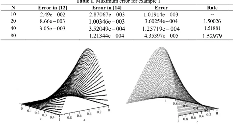
10 20 40 80

Figure 1. C

Results our schemes

cheme (21) is Consider the

ds, T. x 1.

≤ ≤

2, and T 0.5=

The numeric o M N 10× =

esults are pres

from Table 1 is

3 2

. Our r on reported i any

α

. Comp f table 4, in e more accura r in [14], is

Error in [12]

2.49e 002−

8.66e 003−

3.05e 003−

--

omputational so

s, the follow

demonstrated partial integ

5. Takeh 1=

cal solution

640

× is used sented in Tabl

1 reflect that results are sim n [14], but paring the res

[14], the res ate. For examp

1.00346e 0−

Table 1. Ma

Erro

2.870

1.003 3.520

1.213

olution of probl wing

d by

gro-M, of d as

le 1 the milar our sults sults mple, 03, but the Ψ obt use wh tim thi pre res bec res par sin sta me

aximum error f

or in [14]

067e 003−

346e 003−

049e 004−

344e 004−

lem 2 Figu

t the error in t Example 2. Consider Eq. e following ex where

Ψ

, de

i i 0

(z) ∞ ( 1)

=

=



−

The initial

tained from t ed in [14]. T hich has four me. The accur s problem w esents rates o sults are simi cause we us sults are prese

In this articl rtial integro-ngular kernel ability and L2 ethod. In this

for example 1

Erro

1.01914e 3.60254e

1.25719e

4.35397e

ure 2. Computa

this paper is 3

. (1) when _α xact solution u

enotes the enti

1 i

3 ( i 1) z

2

−

Γ +

and bound the exact solu he authors of th-order accu racy of our m with several v

f convergenc ilar to the nu

ed the same nted in Table

Discu

e, a compact differential e

for any0< α

norm converg study, Crank– or 003 − 004 − 004 −

e 005−

tional solution

3.60254e 004−

1 2

α = and μ

5

u(x, t)= Ψ π

ire function

.

dary conditi ution. This te f [14] propos uracy in spac method is teste values of ste ce in time for numerical solu

e method. Th 2.

ussion

t difference s equation wit

1

α < , is con rgence is prov –Nicolson tim Rate -- 1.50026 1.51881 1.52979

of problem 2

4 .

0

= β = , with

5 3_{t sin( x).π}

(44)

ions can be st problem is sed a scheme ce and 3₂ in ed by solving eps size and rT 0.5= . Our ution in [14] he numerical

used to appro trapezoidal m term. The co space. The m solutions of

1

μ =

, and theoretical re rates in time

oximate the d method is use onvergence ord

method was t two different

,

0

β μ =

, b

esults. What’ e will increase

N

20

8.

40

3.

80

1.

160

4.

320

1.5

640

5.

Figure 3. Num

Figure 4. Num

differential ter ed to approxim

der is

2

− α

,

tested against t examples, w both example s more by in e at a steady

Error in [14]

.93117e 002

−

.21568e 002

−

15715e 002

−

.16970e 00

−

50417e 00

−

.46742e 004

−

merical approx

merical approxi

rm and a prod mate the integ

in time and 4 t exact refere where

β =

0

es supported ncreasing

N

,

rate. In additi

Table 2. Ma

Rat

2

2

1.

2

1.4

3

1.

03

1.

4

1.

imations are co

imations are com

duct gral 4 in ence and our

the ion,

num mo wo by

val

aximum error f

te in [14]

--

47372

47455

47256 47098 46004

ompared with ex

mpared with ex

merical resul ore accurate t orth mentionin

Matlab.

We would l luable comme

for example 2

Erro

9.05317e

3.19954e

1.13096e

3.99814e

1.41360e

5.00614e

xact solution (4

xact solution (44

ts presented than those re ng that our co

Acknowl

like to thank ents and helpf

or

e 003

−

e 003

−

e 003

−

e 004

−

e 004

−

e 005

−

44) of problem 2

4) of problem 2

in the prese eported in [1 omputations a

ledgment

k both refere ful suggestion

Rate

--

1.50055

1.50031

1.50014

1.49995

1.49760

2 forN 80= .

2 forN 160₌ .

ent study are 2, 14]. It is are performed

ees for their ns which have e s d

improved the paper.

References

1. Jangveladze T., Kiguradze Z. and Neta B. Numerical Solutions of Three Classes of Nonlinear Parabolic Integro-Differential Equations, Academic Press, New York., (2016).

2. Dumitru B., Darzi R. and Agheli B. New study of weakly singular kernel fractional fourth- order partial integro-differential equations based on the optimum q-homotopic analysis method, J. Comput & Appl. Math.,320: 193-201 (2017).

3. Babaaghaie A. and Maleknejad K. Numerical solutions of nonlinear two-dimensional partial Volterra integro-differential equations by Haar wavelet, J. Comput & Appl. Math., 317: 643-651 (2017).

4. Canuto C. and Quarteroni A. Approximation results for orthogonal polynomials in Sobolev spaces, Math. Comp.,

38: 67-86 (1982).

5. Lakestani M., Nemati Saray B. and Dehghan M. Numerical solution for the weakly singular Fredholm integro-differential equations using Legendre multiwavelets, J. Comput. & Appl. Math., 235(11): 3291-3303 (2011). 6. Tahami M., Hemmat A. A. and Yousefi SA. Numerical

solution of two-dimensional first kind Fredholm integral equations by using linear Legendre wavelet, Int. J. Wavel. Multi. Resolu.& Inf. Proce.,14(01): 1-20 (2016).

7. Lopez-Marcos J.C. A difference scheme for a nonlinear

partial integro-differential equation, SIAM J. Numer. Anal.,

27: 20–31(1990).

8. Xu D. On the discretization in time for a partial integro-differential equations with a weakly singular kernel I: smooth initial data, Appl. Math. Comput. 58: 1–27 (1993). 9. Xu D. On the discretization in time for a partial

integro-differential equations with a weakly singular kernel II: nonsmooth initial data, Appl. Math. Comput., 58: 29–60 (1993).

10. Singh S., Patel V. K., Singh V. K. and Tohidi E. Numerical solution of nonlinear weakly singular partial integro-differential equation via operational matrices, Appl. Math. & Comput., 298: 310-321 (2017).

11. Fakhar-Izadi F. and Dehghan M. Space–time spectral method for a weakly singular parabolic partial integro-differential equation on irregular domains, Comput. &

Math. with Appl., 67(10): 1884–1904 (2014).

12. Tang T. A finite difference scheme for a partial integro-differential equations with a weakly singular kernel, Appl.

Numer. Math., 11: 309–319 (1993).

13. Chen H. and Xu D. A compact difference scheme for an evolution equation with a weakly singular kernel, Numer.

Math. Theory Methods Appl., 4: 559–572(2012).

14. Luo M., Xu D. and Limei L. A compact difference scheme for a partial integro- differential equation with a weakly singular kernel, Appl. Math. Modelling., 39(2): 947-954 (2015).