Studying Transition Behavior of Neutron Point Kinetics
Equations Using the Lyapunov Exponent Method
M. Seidi
*1, R. Khodabakhsh
2, S. Behnia
31Department of Physics, Faculty of Sciences, Ilam University, P.O.Box: 516-69315, Ilam, Islamic
Republic of Iran
2Department of Physics, Faculty of Sciences, Urmia University, P.O.Box:165-57153, Urmia, Islamic
Republic of Iran
3Department of Physics, Urmia University of Technology, P.O.Box:419-57157, Urmia, Islamic
Republic of Iran
Received: 3 October 2015 / Revised: 30 January 2016 / Accepted: 16 February 2016
Abstract
The neutron density is one of the most important dynamical parameters in a
reactor. It is directly related to the control and stability of the reactor power. Any
change in applied reactivity and some of dynamical parameters in the reactor causes a
change in the neutron density. Lyapunov exponent method is a powerful tool for
investigating the range of stability and the transient behavior of the reactor power. In
contrast to the other linear stability methods, this method can be used for large
perturbations and is not needed to construct Lyapunov function. In this work, the
range of stability using Lyapunov exponent method is evaluated for neutron point
kinetics equations with six-groups delayed neutrons. Here, effects of four set of
applications, namely, step, ramp, sinusoidal, and temperature feedback reactivities on
power reactor were investigated with Lyapunov exponent method. The results of
qualitative analysis were compared with traditional methods and were in good
agreement with other works.
Keywords:Temperature feedback; Neutron density; Delayed neutron; Lyapunov exponent.
*Corresponding author: Tel: +988432227204; Fax: +988432227014; Email: [email protected]
Introduction
The dynamic behavior of the reactor can be described via a set of ordinary differential equations known as the neutron point reactor kinetics (NPK) equations [1, 2]. NPK equations describe the variation of in neutron population due to the change of reactivity [2]. The neutron density and the delayed neutron precursor concentration are the most important parameters to be studied, for the purpose of safety and the transient
behavior of the reactor power [3]. These parameters are directly affected by reactivity [4,5].
Lyapunov exponent method [4, 11-13] are the most important methods for nonlinear stability analysis. Lyapunov second method is based on the construct of Lyapunov function for which there are several methods such as Aizerman, Szego, Rosen, variable gradient methods, etc, but there is no systematic method for the construction of this function [8, 11, 13]. Some of the researchers- Fu, Chen, Ergen, etc have used this method [4, 12, 13]. While, for Lyapunov exponents method there is no such problem, so another important method for analyzing and diagnosing instability of nuclear reactors is the spectrum of Lyapunov exponents method, that is based on eigenvalues and eigenvectors of the Jacobian matrix [14-16]. Estimating Lyapunov exponents, which is one of the most important problems of the control theory, has been investigated in the following papers: [17] for discrete time varying linear systems, [18] for continuous time linear systems and [19] for discrete stochastic linear systems. Lyapunov exponents describe necessary and sufficient conditions for asymptotic stability in the linear systems [19]. So, Lyapunov exponent method in the nonchaotic systems can be used for the analysis of stability.
The purpose of the present study is to introduce the mean Lyapunov exponent approach on stability analysis of NPK equations in nuclear reactors with multi-group delayed neutron in the presence of step, ramp, sinusoidal, and temperature feedback reactivities.
This paper is organized as follows. In Sec. 2, a brief description of NPK equations is presented. In Sec. 3, analysis tools are reviewed and finally, the authors are discussed and interpreted the results.
Materials and Methods
In this section we introduce neutron point kinetic equations and Lyapunov exponent method for analysis reactor dynamics.
II-1. Neutron point kinetic equations
NPK equations by considering the temperature feedback reactivities are the stiff non-linear ordinary differential equations [20]. The general form of the equations with m-group delayed neutron precursors is [21-23]:
(1)
1 m
i i i
i i
i i
dn t
t
n t
c t
q t
dt
l
dc t
n t
c t
dt
l
Where
t
is the net reactivity which is the sum of external reactivity (ext
t ) and feedback reactivity
f
t
[24].n t
is the neutron density,c t
i
is the concentration of precursor delayed neutrons,
i is the relative fraction ofi th
group delayed neutron,
is the total effective fraction of delayed neutrons,l
is the prompt neutron generation time,
i is thei th
group constant decay, andq t
is the external neutron source. The effects of arising from the temperature feedback reactivities can be written as [1, 25, 26]:(2)
t
0T t T
0
Here,
is the temperature coefficient of reactivity,0
is initial reactivity,T t
is the temperature of the reactor, andT
0 is the initial temperature of the reactor. After the reactivity
0 is inserted into the reactor, the power responds quickly and the adiabatic model can be used for the calculation of reactor temperature as follows [8]:
c
dT t
k n t
dt
(3)Where,
k
c is the reciprocal of the thermal capacity of the reactor core.II-2. Analysis Tools
In this study we were focused attention on dynamical systems described by a set of ordinary differential equations particularly NPK equations with six group delayed neutron.
though an m dimensional system has m Lyapunov exponents, in most applications it is sufficient to compute only the Lyapunov exponents.
The Lyapunov exponents are defined as follows: Consider two nearest neighboring points (usually the nearest) in phase space at time
0
andt
, with distances of the points in thei th
direction
d
i
0
and
i
d t
, respectively. The Lyapunov exponent is then defined through the average growth rate
i of the initial distance,
2
1
lim log
0
i i t
i
d t
t
d
(4)The Lyapunov exponents for a region of N-dimentional state space near a fixed point are the characteristic values
i that of fixed point.If
iState Space
i0
, then the trajectories approach the fixed point exponentially.If
iState Space,
i0
, then the trajectories repelled from the fixed point exponentially [30].Commonly, Lyapunov exponents (
i) can be extracted by observed signals in the following different method:● Based on the opinion of following the time-evolution of nearby points in the state space.
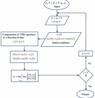
● Based on the estimation of local Jacobi matrices. The first method is usually called Wolf algorithm [31] and it only provides an estimation of the largest Lyapunov exponent. The second method is capable of estimating all the Lyapunov exponents. Using one of these methods, the Lyapunov exponent is calculated rather than a given control parameter. So, there is a little increase in the value of the control parameter and the Lyapunov exponent is calculated for the new control parameter. By continuing this method the Lyapunov exponent spectrum of the point reactor kinetics is
plotted versus the control parameter. In this study, for calculating Lyapunov exponent spectrum was applied Wolf algorithm. This algorithm is shown in Fig.1. According to the Fig.1, we have solved the NPK equations for a arbitrary value of the control parameter (
i) for two initial condition
n
i0 ,
m
i0
n
i0
rand
(1,1),
1,
R
which are very close to each other. Next we have calculateed time series depends on the neutron density that is
i
n t
and
i
m t
. Finally by using the following relation, we have calculated Lyapunov exponent. (5)
2 21
1
lim log
lim log
0
0
0
i i i
i t t
i i i
d t
m t n t
t
d
t
m
n
Results
Here, we study the dynamical behavior of systems Eqs.1 and 3 by calculating their Lyapunov exponents. The set of all Lyapunov exponents of discrete time varying linear systems is called the spectrum of this system (
1, , ,
2
n
) [17]. According to thetheorem of Oseledec, the almost certain stability of the trivial solution of a system can be determined by the largest Lyapunov
max; i.e., when
0
the trivial solution is almost certainly stable and when
0
the trivial one unstable [18]. All of the coordinates in this phase space are given as follows:n t
,c t
1
,c t
2
,
3
c t
,c t
4
,c t
5
andc t
6
. If we want to count of the effect of temperature feedback another coordinate,
T t
is added too. Therefore stability analysis should be followed with the eight Lyapunov exponents
1, , ,
2
8
. It is impossible to obtain thesequantities analytically. Therefore numerical and estimation methods are required for their approximation [18]. Here, numerical calculations have been done with
45
ODE
method. Initial conditions are [3, 20, 21, 32]:0
0
1,
0i ii
n
n
c
l
(6)The data in this study are taken from references [3, 20, 32]. In the following each reactivity will be discussed in a subsection.
III-1. Step Reactivity
We study the dynamical behavior of NPK equations with six-groups delayed neutrons for step reactivity with steps
,
0.5
,0.5
and
. Lyapunov exponent method, is applied to the solving and the stability analysis of NPK equations in the thermal reactor with the following parameters [3, 20]:1 1
0.0127
s
, 12
0.0317
s
, 13
0.115
s
,1 4
0.311
s
,
5
1.4
s
1,
6
3.87
s
1,0.0005
l
s
,
1
0.000285
,
2
0.0015975
,3
0.00141
,
4
0.0030525
,
5
0.00096
,6
0.000196
and
0.0075
.Numerical calculations have been performed with
45
ODE
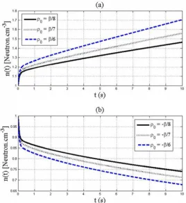
method and relative errors are compared with the exact values of the neutron density (See Table 1) [3, 33]. For positive and negative step reactivities, it can be observed from Figure 2a and 2b, that the neutron density gradually increased andTable 1.The neutron density and relative error of the thermal reactor with step reactivity [3].
Exact RK(ODE45)
h=01 GAEM h=01 AEM h=01 TSM h=01 t0(s)
ρ0($)
0.5206043 0.4333335 0.2361107 0.6989252 0.6070536 0.3960777 1.533113 2.511494 14.21503 2.515766 10.36253 32.18354 6
1.4 10
6
1.85 10
7
9.74 10
6
1.43 10
6
1.6 10
6
1.01 10
7
6.52 10
6
1.11 10
6
1.26 10
6
1.19 10
0.0
7
1.24 10 0.0 0.0 0.0 0.0 0.0 0.0 0.0 0.0 7
7.53 10
0.0 0.0
7
3.11 10
7
1.92 10 0.0 0.0
7
1.43 10 0.0 0.0 0.0 0.0
7
7.53 10
0.0 0.0
7
3.11 10
4
2.2 10 0.0 0.0
6
3.15 10 0.0 0.0 0.0
7
decreased respectively. According to Table 2, in long term
t
, all of the Lyapunov exponents for negative steps (
and
0.5
) are negative. It means that NPK equations are stable in the three dimensional space. So, the neutron density was decreased during time and reactor goes into shutdown. The step reactivity with steps
and0.5
have a positive Lyapunov exponent, (See Table 2). In thissituation, the fixed points of NPK equations with these steps are unstable so, the neutron density will be increased exponentially and reactor with these reactivities cannot remain in critical state [8].
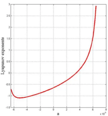
Figure 3, shows the results of Lyapunov exponent method with respect to step reactivity in short term (
t
10
s
). Thus the transient behavior of reactor is stable for
0
0.003156
in short term (t
10
s
). Figure 2.The neutron density as a function of time for three cases of thepositive step reactivity (a), and three cases of the negative step reactivity (b).
Table 2.Lyapunov exponent with respect to time for step reactivity.
-30.2281 -22.8087 -8.4932 -4.3845 -3.8161
-3.7964 -3.6107 -2.4761 -1.3115
-1.2830 -1.0939 -0.7320 -0.2475
-0.2283 -0.1601 -0.1395 -0.0980
-0.0896 -0.0283 -0.0119 -0.0258
-0.0222 -0.0134 -0.0131 -0.0124
-0.0116 0.1725 2.0443 -1
-0.5 0.5 1
Table 3.Lyapunov exponent with respect to time for ramp rate reactivity.
-159.0096 -158.9926 61.7751 158.3794 -3.8656
-3.7964 97.2085 186.8532 -1.31920
-1.2830 97.0994 186.1184 -0.3051
-0.2283 95.5988 184.2730 -0.1137
-0.0896 109.6477 193.9540 -0.0311
-0.0222 9.1515 43.6724 -0.0128
-0.0116 155.2998 239.3204 -0.01
-0.1 0.1 0.01
7
6
5
4
3
2
1
0
$
7
6
5
4
3
2
1
III-2. Ramp Reactivity
The analyses are presented for the thermal reactor with the following parameters [3, 20]:
1 1
0.0127
s
, 12
0.0317
s
, 13
0.115
s
,1 4
0.311
s
, 15
1.4
s
, 16
3.87
s
,0.00002
l
s
,
1
0.000266
,
2
0.001491
,3
0.001316
,
4
0.002849
,
5
0.000896
,6
0.000182
and
0.007
.Regarding the results listed in Table 3, the reactor for all of the negative values of ramp rate reactivities
r
0
is stable in long term, and unstable for all of the positive values of ramp rate reactivities
r0
. Thus, forr
0
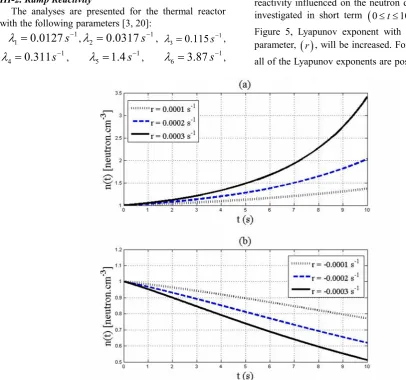
, neutron density reduces gradually, and in long term, reactor goes into shutdown (see Fig. 4b). For0
r
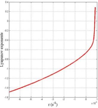
, the neutron density rises rapidly and in the same vein, the period of reactor decreases. Therefore, reactor control will be problematic (see Figure 4a). Numerical results listed in Table 4 imply that.Numerical calculations are performed and compared with TSM, GAEM and Pade methods. Regarding Table 4 the results are in good agreement [20,21]. Ramp rate reactivity influenced on the neutron density behavior is investigated in short term
0 t 10s
. According to Figure 5, Lyapunov exponent with respect to control parameter,
r , will be increased. Forr
0.000798
, all of the Lyapunov exponents are positive so, system isFigure 3.Variation of the Lyapunov exponents with respect to the step reactivity.
unstable (see Figure 5). In long term, the boundary of
stability tend to become zero
r
0
. III-3. Sinusoidal ReactivityIn this subsection, sinusoidal reactivity, 2 sin t a , has been investigated, where
anda
are respectively periods and amplitude of sinusoidal reactivity. It is applied to the thermal reactor with the following parameters [32]:
1 1
0.0124
s
, 12
0.0305
s
, 13
0.111
s
,1 4
0.301
s
, 15
1.14
s
, 16
3.01
s
,0.00003
l
s
,
1
0.000214
,
2
0.001423
,3
0.001247
,
4
0.002568
,
5
0.000748
,6
0.000273
and
0.006473
.The variation of Lyapunov exponents with respect to time have been shown in Table 5. In long term the reactor is unstable for all of the values of amplitude
a
and period
of reactivity. It means that the density of neutron will be increased exponentially (see Figures 6a and 6b).Table 4.The neutron density of the thermal reactor with positive and negative ramp rate reactivity [3].
Ramp reactivity with r 0.1 $
s1
45
0.0001
ODE
h
0.001
Pade h
0.1
GAEM h
0.0001
TSM h
t s
1.3382 2.2285 5.5821 42.7867 54.5117 10
1.3382 2.2284 5.5820 42.786
5
4.5116 10
1.3382 2.2284 5.5820 42.786
5
4.5116 10 1.3382
2.2284 5.5822 42.789
5
4.5143 10
2 4 6 8 10
Ramp reactivity withr 0.1 $
s1
45
0.0001
ODE
h
0.001
Pade h
0.1
GAEM h
0.0001
TSM h
t s
0.792016 0.613021 0.474059 0.369168 0.290653 0.792007 0.613018 0.474058 0.369169 0.290654 0.792007 0.613020 0.474065 0.369172 0.290653 0.792001 0.613018 0.474058 0.369169 0.290654 2 4 6 8 10Table 5.Lyapunov exponent with respect to time for different values amplitude ,(a), and period ,(
s
), of the sinusoidal reactivity. 7
6
5
4
3
2
1
s
-216.1836 -216.1598 -216.0854 -216.0374 -2.8960 -2.8960 -2.8959 -2.8959 -1.0228 -1.0229 -1.0228 -1.0228 -0.1935 -0.1938 -0.1938 -0.1938 -0.0647 -0.0646 -0.0647 -0.0648 -0.0142 -0.0142 -0.0142 -0.0143 0.0005 0.0008 0.0010 0.0011 1 30 70 100 7
6
5
4
3
2
1
$
a
-216.1830 -216.1886 -216.2451 -217.3801 -2.8961 -2.8947 -2.8832 -2.7800 -1.0230 -1.0215 -1.0097 -0.9281 -0.1936 -0.1925 -0.1835 -0.1517 -0.0648 -0.0637 -0.0547 -0.0223 -0.0142 -0.0141 -0.0136 -0.0129 0.0003 0.0017 0.0169 0.9158 0.1 0.2 0.5 1In short term, the reactor can be stable or unstable. For example, the neutron density in 10 s with
1
s
and
a
0.00073
will be decreased (see Table 6). In this range of time reactor is stable. Lyapunov exponents with respect to control parameters are shown in Figures 7 and 8. Figure 7, shows that in the range of1
s
100
s
the reactor is stable. According to Figure 8, in the range of
a
for0.0034522
a
reactor is stable.III-4.Temperature Feedback Reactivity
To complete the analysis, we now consider the NPK equations in presence of temperature feedback reactivity with the following parameters [3,20,21]:
1 1
0.0124
s
, 12
0.0305
s
, 13
0.111
s
,1 4
0.301
s
, 15
1.13
s
, 16
3.0
s
,0.00005
l
s
,
1
0.00021
,
2
0.00141
,3
0.00127
,
4
0.00255
,
5
0.00074
,6
0.00027
,
0.00645
,
0.00005K
1 andk
c
0.05
MW s K
1 1 1.Table 7 shows that all of the Lyapunov exponents are negative for various control parameters. Therefore, system is stable in long term
t
.Figures 9a, 9b and 9c illustrate the change in the neutron density as a function of time for different values of initial reactivity, temperature coefficient of reactivity and the reciprocal of the thermal capacity of reactor, respectively. In these Figs, the neutron density is increased until tend to the maximum point and
Figure 6. The neutron density as a function of time for three cases of the period of sinusoidal reactivity (a), and three cases of the amplitude of sinusoidal reactivity (b).
Table 6.The neutron density of the thermal reactors with sinusoidal reactivity [31].
Sinusoidal reactivity with
a
0.00073
و
1
s
45 0.001 ODE h
Hansen
0.01
DM h
t s
1.12394 1.16889 1.07448 0.95383 0.90735 0.98468 1.12396
1.16880 1.07442 0.95380 0.90737 0.98464 1.12351
1.16816 1.07429 0.95527 0.90454 0.98172 1
decreased until going into zero, due to the effects of temperature feedback reactivity. So, reactor goes into stability.
Table 8, illustrate the response of the neutron density to increase initial reactivity. Numerical calculations with ODE45 are performed and compared with TSM, GAEM and NAM methods. The results are in good agreement [20, 21]. In this work the transient behavior of reactor for range of time
0
t
350
s
and initial reactivity
0
0
2
are considered. According to Fig. 10, all of the Lyapunov exponents with respect to initial reactivity are in the negative range. Therefore, in short term reactor is stable. By changing some dynamical parameters in the reactor such ask
c and
, reactor power can be changed, so here we considered the effectof changing these two parameters using Lyapunov exponent method. Figure 11, imply that the variation of Lyapunov exponents with respect to
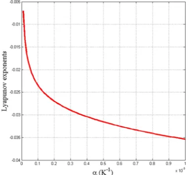
parameter. They are negative in the range of0.00001
0.001
and
0 t 350s
, therefore reactor goes into stability (see Table 7). Figure 12, shows that the variation of Lyapunov exponents with respect tok
c parameter are negative in the range of 0.001kc0.1and
0
t
350
s
. The results of Table 7, are in good agreement with the results of Figures 10, 11 and 12.Discussion
Predicting the dynamic behavior of a nuclear reactor
Figure 7. Variation of the Lyapunov exponents with
respect to the period of sinusoidal reactivity. Figure 8.to the amplitude of sinusoidal reactivity.Variation of the Lyapunov exponents with respect
Table 7.Lyapunov exponent with respect to time for different values control parameters, with temperature feedback reactivity.
due to changes in the parameters of dynamical systems is very important. Lyapunov exponent method is a powerful tool that can help to determine the range of linear and nonlinear systems stability for the changes control parameters of the system. In this work the influence of step, ramp, sinusoidal and temperature feedback reactivities on stability and the neutron of
density with Lyapunov exponent method were investigated, also the analysis of Lyapunov exponent respect to time for reactivities above in long-term scale (t → ∞) was studied. In order to validate the method, the neutron density changes due to changes in the parameters of dynamical systems with ODE45 method was carried out and the results of compared withPade,
Figure 9.The neutron density as a function of time for three cases of the temperature coefficient of reactivity (a), three cases of the reciprocal of the thermal capacity of the reactor core (b), and three cases of the initial reactivity (c).
Table 8.The peak of the neutron density with temperature feedback reactivity [20]. Time of the peak The peak of the neutron density
45
ODE
NAM
GAEM
TSM
45
ODE
NAMGAEM
TSM
0 $
28.293 0.954 0.317 0.168 0.099 28.293
0.953 0.317 0.168 0.098 28.293
0.953 0.317 0.168 0.098 8.293
0.953 0.317 0.168 0.098 45.75243
807.8676 8020.795 43020.82 167738.9 45.75240
807.8666 8020.916 43025.93 167856.6 45.75212
807.8672 8020.919 43024.69 167800.4 45.75429
807.8765 8020.848 43021.00 167739.3 0.5
TSM, GAEM, NAM, DM, and Hansen methods [3,20,32]. The results are in good agreement with each other, so theODE45 method can be used instead of the above methods. The quantitative results from ODE45 method, confirm the qualitative results obtained from Lyapunov exponent method.
References
1. Hamada Y. M. Confirmation of accuracy of generalized power series method for the solution of point kinetics equations with feedback,Ann. Nucl. Energy55: 184-193 (2013).
2. Yamoah S., Akaho E. H. K., & Nyarko B. J. B. An accurate solution of point reactor neutron kinetics equations of multi-group of delayed neutrons,Ann. Nucl. Energy54: 104-108 (2013).
3. Nahla A. A. Analytical solution to solve the point reactor kinetics equations, Nucl. Eng. Des. 240: 1622-1629 (2010).
4. Fu L. Z.. Nuclear Reactor Kinetics.Atomic Energy Press, Beijing, pp. 81-115. ISBN 7-5022-0002-9 (in Chinese) (1998).
5. Li F. Y., Chen Z., & Liu Y. Research on stability of a reactor with power reactivity feedback, Prog. Nucl. Energy67: 15-17 (2013).
6. Lewins J. D., & Ngcobo E. N. Property discontinuities in the solution of finite difference approximations to the neutron diffusion equations, Ann. Nucl. Energy23: 29-34 (1996).
7. Munoz-Cobo J. L., Garca C., Escriva A., & Melara J. Reactivity calculation in the frequency domain for BWR stability codes,Ann. Nucl. Energy35: 1185-1198 (2008). 8. Hetrick D. L.Dynamics of Nuclear Reactors. American
Nuclear Society, La Grange Park (1993).
9. Della R., Alhassan E., Adoo N. A., Bansah C. Y., Nyarko B. J. B., & Akaho E. H. K. Stability analysis of the Ghana Research Reactor-1 (GHARR-1),Energy Convers. Manage.74: 578-593 (2013).
10. Seborg D. E., Edgar T. F., Mellichamp D. A. Process dynamics and control. 2nded.John Wiley and Sons Inc (2004).
11. Ergen W. K., Lipkin H. J., & Nohel J. A. Applications of Lyapunovs second method in reactor dynamics.J. Math. Phys.36: 36-48 (1957).
12. Chen W. Z., Kuang B., & Guo L. F. New analysis of prompt supercritical process with temperature feedback.
Nucl. Eng. Des.236: 1326-1329 (2006).
13. Slotine J. J. E., & Li W. Applied Nonlinear Control, Prentice Hall Englewood Cliffs, New Jersey (1991). 14. Khoda-bakhsh R., Behnia S., & Jahanbakhsh O. Stability
analysis in nuclear reactor using Lyapunov exponent,
Ann. Nucl. Energy35: 1370-1372 (2008).
15. Suzudo T. Application of a nonlinear dynamical descriptor to BWR stability analyses,Prog. Nucl. Energy
43: 217-223 (2003).
16. Shayesteh M., Behnia S., & Abdi Saray A. Criticality calculations in a nuclear reactor by using the Lyapunov exponent method,Ann. Nucl. Energy43: 131-135 (2012). 17. Czornik A., & Nawrat A. On new estimates for
Figure 10. Variation of the Lyapunov exponents with respect to the initial reactivity.
Figure 11. Variation of the Lyapunov exponents with respect to the temperature coefficient of reactivity.
Lyapunov exponents of discrete time varying linear systems,Autom.46: 775-778 (2010).
18. Rong W., Meng G., Wang X. D., Xu W., & Fang T. Largest lyapunov exponent for second-order linear systems under combined harmonic and random parametric excitations, J. Sound Vibration 283: 1250-1256 (2005).
19. Verdejo H., Vargas L., & Kliemann W. Stability of linear stochastic systems via Lyapunov exponents and applications to power systems,Appl. Math. Comput.218: 11021-11032 (2012).
20. Nahla A. A. Taylors series method for solving the nonlinear point kinetics equations,Nucl. Eng. Des.241: 1592-1595 (2011).
21. Nahla A. A. Numerical treatment for the point reactor kinetics equations using theta method, eigenvalues and eigenvectors,Ann. Nucl. Energy38: 2810-2817 (2011). 22. Nahla A. A. An efficient technique for the point reactor
kinetics equations with Newtonian temperature feedback effects,Prog. Nucl. Energy85: 756-763 (2015).
23. Bogado Leite S. Q., PalmaD. A. P., Tullio de Vilhena M.& Bodmann B. E.J.Analytical representation of the solution of the point reactor kinetics equations with adaptive time step, Prog. Nucl. Energy 70: 112-118 (2014).
24. Sathiyasheela T. Power series solution method for solving point kinetics equations with lumped model temperature and feedback, Ann. Nucl. Energy 36:
246-250 (2009)
25. Tashakor S., Jahanfarnia G., & Hashemi-Tilehnoee M. Numerical solution of the point reactor kinetics equations with fuel burn-up and temperature feedback,Ann. Nucl. Energy37: 265-269 (2010).
26. Samuel G., Alexandar S.Nuclear Reactor Engineering. Chapman & Hall, Inc (1981).
27. Ott E.Chaos in dynamical system, Cambridge university pess, Canada (1993).
28. West B. J., Goldberger A. L., Rouner G., & Bhar-gava V. Nonlinear dynamics of the heartbeat: I. The AV junction: Passive conduit or active oscillator?,Phys. D17: 198-206 (1985).
29. Wolf A., Swift J. B., Swinney H. L., Vastano J. A. Determining Lyapunov exponents from a time series,
Phys. D16: 285-317 (1985).
30. Hilborn R. C.Chaos and Nonlinear Dynamics, Oxford University Press, Oxford (2000).
31. Dorfman J. R. An Introduction to Chaos in Nonequilibrium Statistica Mechanics, Cambridge University Press, Cambridge (1999).
32. Petersen C. Z., Dulla S., Vilhena S. T. M. B, & Ravetto P. An analytical solution of the point kinetics equations with time-variable reactivity by the decomposition method,Prog. Nucl. Energy53: 091-1094 (2011). 33. Ramasubramanian K., & Sriram M. S. A comparative
![Table 1. The neutron density and relative error of the thermal reactor with step reactivity [3].](https://thumb-us.123doks.com/thumbv2/123dok_us/19065.2001997/4.595.91.507.563.717/table-neutron-density-relative-error-thermal-reactor-reactivity.webp)
![Table 6. The neutron density of the thermal reactors with sinusoidal reactivity [31]. ](https://thumb-us.123doks.com/thumbv2/123dok_us/19065.2001997/8.595.131.466.631.731/table-neutron-density-thermal-reactors-sinusoidal-reactivity.webp)