A MODIFIED PATCH PROPAGATION-BASED IMAGE INPAINTING USING PATCH SPARSITY

(1)

IJST, Transactions of Electrical Engineering, Vol. 37, No. E2, pp 121-132 Printed in The Islamic Republic of Iran, 2013

A MODIFIED PATCH PROPAGATION-BASED IMAGE

INPAINTING USING PATCH SPARSITY

*

S. HESABI,

**

AND N. MAHDAVI-AMIRI

Faculty of Mathematical Sciences, Sharif University of Technology, Tehran, I. R. of Iran Email: [email protected]

Abstract– We present a modified examplar-based inpainting method in the framework of patch

sparsity. In the examplar-based algorithms, the unknown blocks of target region are inpainted by the most similar blocks extracted from the source region, using the available information. Defining a priority term to decide the filling order of missing pixels ensures the connectivity of the object boundaries. In the exemplar-based patch sparsity approach, a sparse representation of missing pixels is considered to define a new priority term and the unknown pixels of the fill-front patch is inpainted by a sparse combination of the most similar patches. Here, we modify this representation of the priority term and take a measure to compute the similarities between fill-front and candidate patches. Also, a new definition is proposed for updating the confidence term to illustrate the amount of the reliable information surrounding pixels. Comparative reconstructed test images show the effectiveness of our proposed approach in providing high quality inpainted images.

Keywords– Image inpainting, texture synthesis, patch sparsity

1. INTRODUCTION

Restoring damaged regions of an image and removing undesired objects are termed as image inpainting. The basic idea is to fill in the lost or broken parts of an image using the surrounding information in such a way that the final restored result appears to be natural to a not familiar observer.

The applications of image inpainting techniques include removal of scratches in old photographs, repairing damaged regions of an image, removal of undesired objects, and restoration of missing blocks of transmitted images.

The user is to identify the missing or damaged areas objectively, since these areas cannot be easily classified. These specified regions are called inpainting domain or target regions and the undamaged parts, whose information is used to repair the target region, are called source regions.

Recently, several image inpainting approaches have been developed. They are roughly categorized into two main types: PDE (Partial Differential Equation)-based methods, and texture synthesis approaches. PDE-based methods use partial differential equations, which propagate edge information along isophote (i.e., a line with all the points having the same gray value) directions with diffusion techniques. Bertalmio et al. [1] were the first to introduce an image inpainting method. Their PDE-based scheme propagated boundary information of the inpainting domain along the isophote directions. Inspired by the work in [1], two other PDE-based algorithms [2, 3] were proposed by Chan and Shen. The Total Variational (TV) model [2] uses an Euler-Lagrange equation coupled with an anisotropic diffusion to preserve the direction of isophotes. This method does not restore a single object well when its disconnected remaining elements are separated far apart within the target region. The Curvature Driven Diffusion (CDD) model [3] considers geometric information by defining the strength of isophotes. This extended version of the TV approach can inpaint larger damaged regions.

(2)

S. Hesabi and N. Mahdavi-Amiri

IJST, Transactions of Electrical Engineering, Volume 37, Number E2 December 2013 122

A simple inpainting algorithm based on prior models was presented by Roth and Black [4]. They modified the diffusion technique of denoising approaches to learn image statistics from natural images and then applied it to the target region. Noori et al. [22] proposed a method based on bilateral filters which was originally used for image denoising. They iteratively convolved the damaged image with a space variant kernel to restore the thin regions.

In almost all PDE-based algorithms, blurring artifacts may be produced when the missing regions are large and textured. So, these methods perform well on images with pure structures or thin target regions.

To fill in large regions with pure textures, the second class of approaches, texture synthesis techniques were proposed. The common idea in these methods is to duplicate the information on the source region into the target region [5-10]; hence, the texture information is preserved.

Texture synthesis approaches are classified into pixel-based sampling [5-7] and patch-based sampling [8-10] according to the sample texture size. Since the filling process in pixel-based scheme is performed pixel by pixel, the algorithm is very slow. However, the speed of patch-based sampling was greatly improved even though filling in the target region is by blocks of pixels, but discontinuous flaws between neighboring patches still remains.

As natural images usually contain both structure and texture components, Bertalmio et al. [11] decomposed the input image into its structure and texture components and then restored them separately. The final outcome was the sum of two reconstructed components. This method is not appropriate for repairing large and thick damaged regions, because the PDE-based approach being used to construct the structure component often admits blurring artifacts. Criminisi et al. [12] presented an examplar-based inpainting technique to propagate the known patches (i.e., examplars) into the missing ones by ordering the synthesizing process. They can remove large objects from the image according to the defined patch priority values assigned to the pixel. Constructing information on both the structure and the texture characteristics for large and thick damaged regions is a special feature of this method.

Other examplar-based schemes were also proposed [13-15]. Compared with the PDE-based approaches, the examplar-based inpainting algorithms have produced plausible results; however, they appear to fail on repairing other types of structures, such as curves, and are often faced with some artifacts in the output image.

Some approaches based on image sparse representation were also introduced for the inpainting problem [16-19]. In these methods, an image is presented by a sparse combination of an overcomplete set of transformations (e.g., wavelet, contourlet, DCT, etc.), and then the missing pixels are inferred by adaptively updating the sparse representation. In [16], Elad et al. proposed an approach to separate the image into cartoon (structure) and texture components, and then represented the sparse combination of the two obtained components by two incoherent over-complete transformations. Although this approach can effectively fill in the regions with structure and texture, it may fail to repair the structure or might produce smoothing defects similar to the PDE-based approaches. Fadili et al. [17] proposed a sparse representation-based iterative algorithm for image inpainting. They used the Expectation Maximization (EM) framework to consider recovering the missing samples based on representations. The proposed approach in [18] is considered a simple exemplar-based model via global optimization. Hence, some problems associated with progressive fill-ins were avoided. Xu and Sun [19] presented an exemplar-based inpainting method using a patch sparsity representation. They introduced the idea of sparse representation under the assumption that the missing patch could be represented by sparse linear combinations of candidate patches. Then, a constrained optimization model was proposed for the patch inpainting. Nonetheless, at times the edges in the filled regions are not connected properly.

Here, we intend to improve the patch sparsity image inpainting scheme based on the patch propagation scheme proposed in [19].

(3)

A modified patch propagation-based image…

December 2013 IJST, Transactions of Electrical Engineering, Volume 37, Number E2 123

2. PATCH SPARSITY-BASED IMAGE INPAINTING

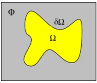
We use the common notations being used in the inpainting literature. The target region, i.e., the region to be filled in, is shown by Ω, and its boundary is denoted by δΩ. The source region, ϕ, which remains fixed throughout the algorithm, supplies samples to fill in the missing regions (refer to Fig. 1).

Fig. 1. Notation diagram: The original image to be filled with target

region , its boundary and the source region

The conventional examplar-based method [12] is as follows.

Algorithm1: A conventional examplar-based method.

Step 1: For each point on the boundary , construct a patch , with in the center of the patch. Step 2: Compute the patch priority : is defined as the product of two terms: a confidence

term , and a data term (see Fig. 2):

. , (1) ∑ _∈ _∩

, . , (2)

where, is the area of , is a normalization factor (e.g., 255 for a typical grey-level image), is a unit vector orthogonal to the boundary at the point , and is an isophote vector. lets linear structures to be synthesized first, and thus propagates securely into the target region, illustrates the amount of the reliable information surrounding the pixel and is initialized to be , ∀ ∈ , and , ∀ ∉ .

Ω δΩ

Φ

Fig. 2. Given the patch for image I, is the normal to the boundary

at , and is the isophote vector

Step 3: Find the patch with the highest priority being filled in with the information extracted from the source region (Fig. 3a).

Step 4: Make a global search on the whole image to find a patch having the most similarity with . Formally,

∈ , (3)

where the distance between two generic patches is simply defined as the sum of squared differences (SSDs) of the already known pixels in the two patches (Fig. 3b).

Step 5: Copy the value of each pixel to be filled in, | ∈ ∩ , using its corresponding position inside (Fig. 3c).

Step 6: Update the confidence term in the area encircled by as follows:

(4)

(a) (b) (c)

Fig. 3. Algorithm 1: (a) The patch with the highest priority is found to be filled in, (b) The most similarity

candidate patches with are determined, e.g. and , (c) The best matching patch in the

candidate set copied into the position occupied by , and thus partial filling of  is achieved

Before discussing our improvement of the patch sparsity inpainting method proposed in [19], we first explain the general steps of the algorithm.

The method investigates the sparsity of image patches and measures the confidence of the patch located at the structure region by the sparseness of its nonzero similarities to the neighbouring patches. The patch with larger structure sparsity is assigned a higher priority for further inpainting. The algorithm can be presented in six steps. Steps 1, 3, 5, and 6 are quite similar to the conventional examplar-based method (Algorithm 1). The priority term in Step 2 is computed in a different way. A sparse linear combination of weighted candidate patches is also used to fill in the missing patch instead of using a single best match in Step 4. Therefore, the steps 2 and 4 of Algorithm 1 are modified as follows:

Step 2: A new definition for patch priority, namely structure sparsity, is proposed. For any selected patch, a collection of neighbouring patches with the most similarities is also distributed in the same structure or texture. Therefore, the confidence of structure for a patch is measured by the sparseness of its nonzero similarities to the neighbouring patches. The patch with more sparsely distributed nonzero similarities is laid on the fill-front due to the high structure sparseness.

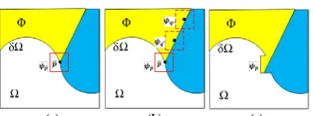
For the patch , located at the fill-front , a neighbourhood window , with the center , is set (refer to Fig. 4a). The sparseness of similarities for the patch is measured by

∑ _, | |

| | (5) where the patch is located in the known region centered at , and , refers to the similarity between and (Fig. 4b), as defined by:

,

(6)

with measuring the mean squared distance of the already known pixels in the two patches, being a normalization constant so that ∑ _, , and being set to 5. Finally,

is defined to be

: ∈ ⊂ (7) The patch priority (or structure sparsity) term is defined as the product of the transformed structure sparsity term and the patch confidence term that is,

, . (8)

where , is a linear transformation taking into the interval , .This transformation scales the structure sparsity variations to be comparable with .

(5)

. Therefore, the unknown pixels in patch is approximated by linear combinations of the , that is,

∑ (9)

where the coefficient vector , , … , is obtained by solving a constrained optimization problem in the framework of a sparse representation (Fig. 4c).

(a) (b) (c)

Fig. 4.The patch sparsity inpainting method proposed in [19]: (a) The neighbourhood window , withthecenter

, is set for the patch

located at the fill-front , (b) To measure the sparseness of similarities for

the similarity between and , , , is computed, (c) The unknown pixels in patch , which

has the highest priority, are filled by linear combinations of the top most similar patches

weighted by coefficients obtained by solving an optimization problem

This optimization problem minimizes the l0 norm of , i.e., the number of nonzero elements in

the vector , with the linearity assumption of the combination.

3. THE PROPOSED METHOD

Our proposed algorithm is given next. We modify steps 2, 4 and 6 to attain better results. Algorithm 2: A modified patch propagation-based image inpainting using patch sparsity.

Step 1: For each point on the boundary , a patch is constructed with as the center of the patch (as in [12] and [19]).

Step 2: To compute the patch’s priority , a stable definition is used as follows:

, , (10)

where the terms , and are the same as the ones defined in [19], and and are the component weights with , and . As illustrated in [20], the confidence value rapidly drops to zero as the filling process goes on. When the dropping effect occurs, error continually propagates to the central part of the reconstructed image, causing noticeable visual artifacts. Therefore, a regularizing transformation is used to control the decreasing rate of the confidence term. We propose using a linear transformation to take into the interval , . Also, the priority term is changed to an additive form instead of a multiplicative form (because the numerical multiplication is effectively sensitive to extreme values, while the additive form has been shown to be more robust with respect to its input and hence more stable).

Step 3: Find the patch with the highest priority to be filled in with the information extracted from the source region (as in [12] and [19]).

Step 4: Perform a global search on the whole image to find the most similar patches. Formally,

arg min _∈ , ,

(6)

where the distance between two generic patches is simply defined as the sum of squared differences (SSDs) of the already known pixels in the two patches.

As a patch may contain texture details, we also include the gradient and divergence differences ( and , respectively) between the already known pixels in the two patches to attain more accuracy. Hence, these added terms cause the preservation of texture properties.

Step 5: Once the most similar patches are found, we use a linear combination of patches to finally obtain the prediction of the missing pixels in (as in [19]).

Step 6: Let ∑ (12)

Denote the unknown pixels in the patch , by a matrix , filled by the corresponding pixels in :

. (13) As illustrated in [19], the coefficients , , … , are obtained by solving the following constrained optimization problem:

‖ ‖

. . ,

, ∈

,

∑ . (14)

The first and the second constraints concern the local patch consistency. The first constraint constrains the estimated patch approximated by the target patch over the already known pixels, and the second one forms the consistency between the newly filled pixels and the neighboring patches in appearance. It measures the similarity between the estimated patch and the weighted mean of the neighboring patches over the missing pixels. The last constraint imposes a normalization summation on the coefficients vector . This constraint is used to achieve invariancy while reconstructing the target patch from its neighboring candidate patches. The parameter is to control the error tolerance, balances the strength of the two first constraints, which is set to 0.25 in our implementation (as in [19]), and _, is defined to be as given in (6).

The local patch consistency constraint can be rewritten in a compact form:

, (15) where,

,

∑ _∈ _, (16)

So, the optimization problem can be formulated as ‖ ‖

. .

(7)

December 201

w [2 w s

Step 7: U

w p B in p Next, we pr

We have im technique [4 To set approach in programs on for the meth As pro equal to 9 [19].

In our Fig. 1, the s to 0.5 and 0 Figure is effective multiplicativ conventiona

Figure [12] and [19

13

which can be 21]. In our with columns olution as

Update the c

where the nu patch . By this defin

n, | ∈ pixel. Hence,

resent our ex

4.

mplemented o 4], conventio up the sam n [12], and th n a laptop w hod in [4] we oposed in [12 9 pixels. Th

proposed alg size of the ne 0.5, respectiv

5 shows the ly sensitive ve form. So, al one.

Fig. 5. The e im

6 shows so 9] for the app

A

e solved in th case, the Gr s , … ,

confidence te

umerator in t

nition, we dif ∩ ; the ne , we can redu xperimental r

IMPLEME

our proposed onal approac me computing

he patch spar with CPU spe ere obtained 2], we applie he parameter

gorithm, the eighbourhoo vely. Also, th e constancy d

to extreme , the obtaine

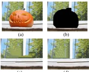
ffect of new d mage, (c) Inpai (d) Inp

ome results o plication of o

modified patch

IJ

he same way ramm matrix

, and

erm in t

the first term

fferentiate be w filled in p uce the rate o

esults.

ENTATION

d method and h [12], and th g environme rsity method ecifications: I

using the co ed the conve rs used in th

size of the p od window, he number of

definition fo values, the d result for t

(a)

(c) definition for t inted image w painted image

obtained by object remov

h propagation-b

IJST, Transacti

y as in Locall x is

1 is a colum

the area enci

∈ ∩

.

m is conside

etween the c pixels do no of error diffu

N AND EXPE

d compared t the patch spa ent, we have d in [19] usin Intel® Core™ ode provided

entional meth he patch spar

patch windo , was se f candidate p or the patch p

additive for this new defi

(b)

(d) the patch prio with the multip with the addit

our method val.

based image…

ions of Electric

ly Linear Em

mn vector of o

ircled by

̂ , ∀ ∈

ered to be th

centered pixe t have inform usion as the f

ERIMENTA

the results wi arsity method e implement ng Matlab 7. ™ i5, 2.4 GH

by the first a hod with the rsity approac

ow was se et to 1111 a

atches, , w priority rm is more finition is bet

rity: (a) Origi plicative form tive form of

in comparis

cal Engineering

mbedding (LL , ones. Then, w

as follows:

∩ Ω

he number of

el, , and the mation as re filling procee

AL RESULT

ith those obta d [19] on sev

ed Algorithm 10.0 instruct Hz, and 4GB author of [4] e patch size ch are the sa

t to 77 pix and the value was fixed to b

. As the num robust and tter than the

nal image, (b)

of , and

son with the

g, Volume 37, N

LE) for data , where X is we have a clo

f known pix

e pixels rece eliable as the eds.

TS

tained by a P veral differen m 2, the con tions and exe B of RAM. T

.

(i.e., size of ame as those

xels. For mos e of and be 21. merical mult more stable result obtain ) Degraded d

proposed m

Number E2 127

reduction s a matrix

osed form

(18)

(19)

xels in the

ntly filled e centered DE-based nt images. nventional ecuted the The results

f ) being e given in

st cases in were set

tiplication e than the ned by the

(8)

IJST, Transac 128 The fir illustrates th patch spars algorithm u As obs even using are more ac similarity m just the co

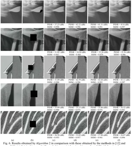
Fig. 6

ctions of Electr

rst and secon he results ob sity method, using the conv

served in Fig the conventi cceptable tha metric is affir onventional

(a) 6. Results obta

[19]: (a) Orig image from (f) Inp

rical Engineeri

nd columns btained from and the la ventional an g. 6, the res ional similar an those illus rmed by com similarity m

(b)

ained by Algo

ginal image, (b m [19], (e) Inpa painted image

S. Hesabi a

ing, Volume 37

are the orig the conventi ast two colu d the newly ults of our p ity metric. V strated in col mparing the fi metric, i.e.,

PSNR = 37.2 SSIM = 0.99

PSNR = 31.8 SSIM = 0.96

PSNR = 31.0 SSIM = 0.98

PSNR = 35.8 SSIM = 0.98

PSNR = 26.5 SSIM = 0.93

(c)

orithm 2 in com

b) Degraded im ainted image b

by Algorithm

and N. Mahda

7, Number E2

ginal and deg ional algorith umns demon

proposed sim proposed alg Visually it is lumns (c) an ifth and sixth

(3), contain

23 (dB) PSNR 94 SSIM

mparison with image, (c) Inp

by Algorithm m 2 using the p

vi-Amiri

graded imag hm, the fourt nstrate the r

milarity metr gorithm are found that t nd (d). Also,

h columns. W n artifacts t

R = 42.22 (dB) = 0.996

R = 34.94 (dB) M = 0.985

R = 42.59 (dB) = 0.996

R = 35.15 (dB) = 0.974

R = 33.02 (dB) = 0.957

(d) h these obtaine ainted image 2 using (3) as proposed simi

es, respectiv th column sh esults obtain ric, respectiv

superior ove he presented robustness o We notice tha hat are not

PSNR = 41.31 (dB SSIM = 0.991

PSNR = 35.26 (dB SSIM = 0.979

PSNR = 42.64 (dB SSIM = 0.992

PSNR = 35.86 (dB SSIM = 0.976

PSNR = 27.88 (dB SSIM = 0.941

(e) ed by the meth

from [12], (d) s similarity me larity metric,

Dece

vely, the thir hows the resu

ned by our vely.

er the two ot d results in c

of the newly at patches ch t well suited

B) PSNR = 43 SSIM = 0.9

B) PSNR = 3 SSIM = 0

B) PSNR = 43 SSIM = 0.9

B) PSNR = 36 SSIM = 0.9

B) PSNR = 26 SSIM = 0.

(f) hods in [12] a ) Inpainted etric, and

(11)

ember 2013

rd column ults of the proposed

ther ones, olumn (e) proposed hosen with d for the

(9)

December 201

neighborhoo more visual

The m the error pr pixel and th rows show our propose confidence Figur

As obs Figure removal. Th respectively patch sparsi 13 od, whereas lly pleasant p modification ( opagation, s he newly fill the original ed method u

term, respec

re 7.docx

Fig. 7. The (b) D fo

served in Fig 8 presents m he first and s y show the im

ity method [1

A

our metric, patches and p (19) for upd

ince the rate ed ones. The

and degrade using the co

tively.

e effect of the Degraded imag

or , and (

g. 7, the resul more examp second rows mages obtain 19] and our p

modified patch

IJ

i.e., (11), c produces bett ating the con e of reliable i

e effect of th ed images, an onventional

new definition ges, (c) Inpain

(d) Inpainted i

lt obtained by ples for the a

show the ori ned by a PDE

proposed alg h propagation-b IJST, Transacti considering tter results. nfidence term information his new defin

nd the third definition (4

(a)

(b)

(c)

(d) n for confiden nted images wi images with th

y the new co application o iginal and de E-based tech gorithm.

based image…

ions of Electric

more proper

m after fillin is controlled nition is show

and fourth r 4) and the n

nce term, ith the conven he new definit

onfidence term of text remov

egraded imag nique [4], th

cal Engineering

rties between

ng in the unk d by the diffe

wn in Fig. 7 ows show th newly propo

: (a) Original ntional definiti

tion for

m is more pl val, scratch r ges, and the t e convention

g, Volume 37, N

n the patche

known pixel ference of the . The first an he images ob osed one (19

l images, tion

lausible. restoration a third to the s nal algorithm Number E2 129 es, selects ls reduces e centered nd second btained by 9) for the

(10)

R a

IJST, Transac 130

Fig. 8. Resu Firs Results of PDE-b algorithm [4]

The original Im

The degraded

Results of conve inpainting metho

Results of patch sparsity approac

Results of our proposed algor

ctions of Electr

ults obtained b st and second results of PD presented i an based

mages

Images

entional od [12]

h ch [19]

rithm

rical Engineeri

PSNR = 36.64 (dB) SSIM = 0.948

PSNR = 28.62 (dB) SSIM = 0.882

PSNR = 37.55 (dB) SSIM = 0.976

PSNR = 37.98 (dB) SSIM = 0.981

by Algorithm 2

rows are the o DE-based techn in the fourth ro nd the last row

S. Hesabi a

ing, Volume 37

(a)

) PS

SS

) PS

SS

) PS SS

2 in compariso original and d nique [4], the ow, the results w demonstrate

and N. Mahda

7, Number E2

(b)

SNR = 34.74 (dB) SIM = 0.959

SNR = 28.15 (dB) SIM = 0.956

SNR = 35.74 dB SIM = 0.979

SNR = 37.06 (dB) SIM = 0.985

on with the on degraded imag

results of con s obtained by es the results o

vi-Amiri

PS SS

PSN SSI

PSN SS

nes obtained b ges, respective nventional inp [19] are illust of our propose

(c)

SNR = 32.69 (dB) SIM = 0.941

SNR = 33.33 (dB) SIM = 0.942

NR = 39.47 (dB) IM = 0.994

NR = 42.54 (dB) IM = 0.996

by the method ely. The third r

ainting metho trated in the fi ed algorithm

Dece ds in [4], [12]

row shows the od [12] are fifth row,

(11)

Roth and Black [4] used the prior models to restore the image; the models have been shown to be useful when images have noise or uncertainty. They proposed a framework for learning image priors. The prior model used in their work was Markov random field (MRF), which assumes an image to be the result of a random process, described by an MRF.

For images in Fig. 8, the size of the patch window was set to 77 pixels and the value of and were set to 0.5 and 0.5, respectively. The size of the neighbourhood window, , was set to 1111, 1919, and 5151 pixels for images (a), (b) and (c), respectively. Also, the number of candidate patches,

, was fixed to be 11, 3 and 25, correspondingly.

We have used the parameters of the approach in [4] unchanged for all the examples considered here. This scheme converted color image to YCbCr color model, and the algorithm was independently applied to all 3 channels. We used a FoE prior with 8 filters of 3×3 pixels. The algorithm inpainted the missing areas by iteratively propagating information. We set the number of iterations to 200.

As seen in Fig. 8, the PDE-based method [4] performs well on piecewise smooth image, Fig. 8 (a), but fails to reconstruct areas containing texture with fine details and tends to blur the inpainted image, Fig. 8 (b) and (c). The conventional algorithm [12] cannot preserve the edge continuity and the texture consistency, and thus produce unpleasant artifacts. The patch sparsity algorithm [19] produces more pleasant results; however, it fails to reconstruct some edges properly.

In contrast, the results obtained by our algorithm appear to be closer to the original image than the ones obtained by the other three methods. Because of the improvement in the priority term, high importance was given to the structures in a more robust way. Also, the proposed similarity metric encompasses more properties of the patches and selects the most visually pleasant ones. Furthermore, the modification in the confidence term after filling in pixels helps reduce the error propagation.

For a quantitative comparison, we computed the peak signal-to-noise ratio (PSNR) and structural similarity (SSIM) values between the original and inpainted images, also observing overall better obtained PSNR and SSIM values by Algorithm 2.

However, similar to [19], our algorithm cannot properly recover large missing areas consisting of structures while the known region doesn’t contain any structure cues. This is a limitation of our algorithm, which needs to be investigated in a future work.

5. CONCLUSION

We presented a modified patch sparsity scheme for inpainting degraded images. Addressing the patch sparsity approach as a robust inpainting method, the suggested modifications lead to an improvement in producing better results. We applied the proposed algorithm to several images and compared the obtained result with those obtained by three other methods. The high visual quality of the results obtained by our approach affirmed the effectiveness of the proposed algorithm.

In future, we will also investigate the effects of varying patch sizes and try to select an optimal size. Moreover, the number of sufficient candidate patches would be explored since it has a direct impact on the computational time of inpainting.

Acknowledgment: The authors sincerely thank Stefan Roth for distributing the inpainting code and also

(12)

REFERENCES

1. Bertalmio, M., Sapiro, G., Caselles, V. & Ballester, C. (2000). Image inpainting, computer graphic

(SIGGRAPH), pp. 417–424.

2. Chan, T. F. & Shen, J. (2002). Mathematical models for local non-texture inpainting. SIAM Journal of Applied

Mathematics, Vol. 62, No. 3, pp.1019–1043.

3. Chan, T. F. & Shen, J. (2001). Non-texture inpainting by curvature-driven diffusions. Journal of Visual

Communication and Image Representation, Vol. 12, No. 4, pp. 436-449.

4. Roth, S. & Black, M. J. (2009). Fields of experts. International Journal of Computer Vision Computer, Vol. 82,

No. 2, pp. 205-229.

5. Ashikhmin, M. (2001). Synthesizing natural textures. ACM Symposium on Interactive 3D Graphics, pp. 217–

226.

6. Efros A. A. & Leung, T. K. (1999). Texture synthesis by non-parametric sampling. IEEE International

Conference on Computer Vision, Vol. 2, pp. 1033–1038.

7. Wei, L. Y. & Levoy, M. (2000). Fast texture synthesis using tree-structured vector quantization. Proc. ACM

Conf. Comp. Graphics, pp. 479–488.

8. Efros, A. A. & Freeman, W.T. (2001). Image quilting for texture synthesis and transfer. Proc. ACM Conf. Comp.

Graphics (SIGGRAPH), Eugene Fiume, pp. 341–346.

9. Freeman, W. T., T. R. Jones and E.C. Pasztor, “Example-based super-resolution”, IEEE Computer Graphics and

Applications, vol. 22, issue 2, pp. 56–65, 2002.

10. Liang, L., Liu, C., Xu, Y., Guo, B. & Shum, H. Y. (2001). Real-time texture synthesis using patch-based

sampling. ACM Trans. on Graphics, Vol. 20, No. 3, pp. 127–150.

11. Bertalmio, M., Vese, L., Sapiro, G. & Osher, S. (2003). Simultaneous structure and texture image inpainting.

IEEE Trans. Image Process., Vol. 12, pp. 882–889.

12. Criminisi, A., Perez, P. & Toyama, K. (2003). Object removal by exemplar based inpainting. IEEE Computer

Vision and Pattern Recognition (CVPR), Vol. 2, pp. 721–728.

13. Drori, I., Cohen-Or, D. & Yeshurun, H. (2005). Fragment-based image completion. ACM Trans. Graph., Vol.

22, No., pp. 303–312.

14. Hung, J. C., Hwang, C. H., Liao, Y. C., Tang, N. C. & Chen, T. J. (2008). Exemplar-based image inpainting

based on structure construction. Journal of Software, Vol. 3, No. 8, pp. 57-64.

15. Wong, A. & Orchard, J. (2008). A nonlocal-means approach to exemplar-based inpainting. Proceeding of IEEE

International Conference on Image Processing, pp. 2600-2603.

16. Elad, M., Starck, J. L., Querre, P. & Donoho, D. L. (2005). Simultaneous cartoon and texture image inpainting

using morphological component analysis. Appl. Comput. Harmon. Anal., Vol. 19, pp. 340–358.

17. Fadili, M. J., Starck, J. L. & Murtagh, F. (2009). Inpainting and zooming using sparse representations. The

Comput. J., Vol. 52, No. 1, pp. 64–79.

18. Wohlberg, B. (2011). Inpainting by joint optimization of linear combinations of examplars. IEEE Signal

Processing Letters, Vol. 18, No. 1, pp. 75–78.

19. Xu, Z. & Sun, J. (2010). Image inpainting by patch propagation using patch sparsity. IEEE Transactions on

Image Processing, Vol. 19, No. 5, pp. 1153–1165.

20. Cheng, W. H., Hsieh, C. W., Lin, S.K., Wang, C.W. & Wu, J. L. (2005). Robust algorithm for exemplar-based

image inpainting. CGIV.

21. Roweis, S.T. & Saul, L. K. (2000). Nonlinear dimensionality reduction by locally linear embedding. Scienc, Vol.

290, pp. 2323–2326.

22. Noori, H., Saryazdi, S. & Nezamabadi-pour, H. (2011). A bilateral image inpainting. Iranian Journal of Science