Christophe Andrieu & Dan Crisan, Editors DOI: 10.1051/proc:071915
PARTICLE FILTER-BASED APPROXIMATE MAXIMUM LIKELIHOOD
INFERENCE ASYMPTOTICS IN STATE-SPACE MODELS
∗Jimmy Olsson
1and Tobias Ryd´
en
1Abstract. To implement maximum likelihood estimation in state-space models, the log-likelihood function must be approximated. We study such approximations based on particle filters, and in par-ticular conditions for consistency of the corresponding approximate maximum likelihood estimator. Numerical results illustrate the theory.
Introduction
By a state-space model is meant a bivariate process (Xk, Yk)k≥1 such that (Xk) is a Markov chain (on some
general state space X) and (Yk) is is a process that depends locally on (Xk) in the sense that given (Xk), (i)
theYk are conditionally independent and (ii) the conditional distribution ofYndepends onXnbut on no other
X-variables. Models with finite state spaceX are often referred to as hidden Markov models. In a state-space model the Markov chain (Xk) is assumed unobservable (or, latent), while the process (Yk) is observable. Hence, all inference etc. must be based on the latter process. State-space models are useful in almost any area where statistical modelling is applied; see the monographs [6, 7] for further reading on the subject in general.
The topic of this paper is parameter estimation in state-space models. The transition kernel Qof (Xk) and
the conditional densitiesg(y|x) of Yk given Xk =xare both assumed to depend on some (finite-dimensional)
parameterθ, which we indicate by writingQθandgθ(y|x) respectively. Typicallyθis naturally divided into two
parts, parametrisingQ andg respectively. To estimateθ from some observed datay1:n = (y1, y2, . . . , yn), the
standard method is maximum likelihood. This approach is non-trivial however, as the likelihood is generally not available in closed form. Indeed, the log-likelihoodn(θ) is typically decomposed as
n(θ) = n
k=1
logpθ(yk|y1:k−1),
where pθ(yk|y1:k−1) is the conditional density of Yk given Y1:k−1. By conditioning on the stateXk and using
the structure of a state-space model, we find that
n(θ) =
n
k=1
log
X
gθ(yk|x)Pθ(Xk ∈dx|y1:k−1), (1)
∗This work was supported by grants from the Swedish Research Council and the Swedish Foundation for Strategic Research.
1 Centre for Mathematical Sciences, Lund University, Box 118, 221 00 Lund, Sweden
c
EDP Sciences, SMAI 2007
where Pθ(Xk ∈ · |y1:k−1) is the predictive distribution, or predictor, of the state Xk given data y1:k−1. This distribution is in general not available in closed form. In the following section we shall study the use of so-called particle filters to approximate these distributions, the resulting approximation of the log-likelihood and its maximiser.
1.
The predictor-filter recursions and particle filters
Writeπθ
k|k−1(·) =Pθ(Xk ∈ · |y1:k−1) for the predictor andπθk|k(·) =Pθ(Xk ∈ · |y1:k) for the so-called filter distribution, or simplyfilter. These distributions are related recursively as
πkθ|k(dx) = gθ(yk|x)π
θ
k|k−1(dx)
Xgθ(yk|x)πkθ|k−1(dx)
(2)
and
πθk+1|k(dx) =
XQθ(x ,dx)πθ
k|k(dx), (3)
respectively. Here (2) is simply Bayes’ formula, while (3) amounts to propagating the filter distribution through the Markov chain dynamics. The recursions are initialised by setting πθ1|0 =ν; the initial distribution of the Markov chain. These recursions in general lack closed-form solutions, with the exceptions of hidden Markov models (the integrals turn into finite sums) and linear Gaussian state-space models (the solution being provided by the Kalman filter).
The literature contains numerous ways to approximate the solution to (2)–(3). Common approaches include the extended Kalman filter, the unscented Kalman filter, spline methods etc. In this paper we will employ so-called particle filters for this purpose. In a particle filter, a collection of particles is used to track the stateXk
of the system, and the predictor and filter distributions are approximated by the empirical distributions of such collections. To make this idea precise, assume that for some indexkwe have available a collection (ξkθ,N|k−1,i)1≤i≤N
of points in X whose empirical distribution πθ,Nk|k−1 is an approximation to πθ
k|k−1. The transformation (2) is
then approximated as follows.
(i) Weighting. Compute unnormalised weights ˜wθ,Nk,i =gθ(yk|ξθ,Nk|k−1,i) and then normalised weightswθ,Nk,i =
˜
wθ,Nk,i /jw˜k,jθ,N.
(ii) Resampling. Create a sample (ξkθ,N|k,i)1≤i≤N by samplingN times independently from (ξkθ,N|k−1,i)1≤i≤N
with weights (wθ,Nk,i )1≤i≤N.
The empirical distribution πkθ,N|k of the sample (ξkθ,N|k,i)1≤i≤N approximates πθ
k|k. The transformation (3) is
approximated as follows.
(iii) Mutation. Create a sample (ξθ,Nk+1|k,i)1≤i≤N by independently samplingξkθ,N+1|k,i fromQθ(ξkθ,N|k,i,·).
The procedure is initialised by letting (ξ1θ,N|0,i)1≤i≤N be an i.i.d. sample of sizeN from the initial distributionν.
The procedure described above is known as the bootstrap particle filter: the mutation of particles follows the system dynamics, and resampling is done multinomially at each step. There is an abundance of variations of this simplest scheme with other strategies for mutation and resampling, and we refer to [1, 3] for extensive coverage of particle filter theory and algorithms.
2.
Assumptions
In this section we give conditions that are assumed to hold throughout the paper. The parameterθis assumed to belong to a parameter set Θ, which is a compact subset ofRdfor somed. The observations (Y
k) arise from a
(A1) The function qθ(x, x) is bounded away from zero and infinity, uniformly inθ,xandx. For ally, the functionθ→Xgθ(y|x)µ(dx) is bounded away from zero and infinity.
The first part of this assumption is typically fulfilled only if X is compact, or at least bounded. It implies that for allθ,Qθ is positive Harris recurrent with a unique stationary distributionγθ. For a stationary version
of the Markov chain, obtained with ν = γθ, and the corresponding state-space model, we write Pθ and Eθ
respectively for the corresponding distributions and expectations. Generally we do assume however that the initial distribution ν is fixed an known; letting ν depend on θ introduces no new principal difficulties, but requires some regularity conditions on the mappingθ→νθ similar to the conditions listed below.
(A2) The function gθ(y|x) is bounded uniformly in θ, x and y, and Eθ0|logb−(Y1)| < ∞ where b−(y) =
infθ
Xgθ(y|x)µ(dx).
(A3) For all x, x and ally, the functions θ→ qθ(x, x), θ→ gθ(y|x) andθ →loggθ(y|x) are continuously
differentiable.
(A4) The gradient∇θlogqθ(x, x) is bounded uniformly inθ,xandx, andEθ0[supθsupx∇θloggθY1(x)]<
∞.
(A5) For some integerp≥1, the expectation
Eθ0
sup
x,x
gθ(Y1|x) gθ(Y1|x)
p
X1=x
is bounded in θ.
(A6) θ=θ0 if and only ifPYθ =PYθ0.
3.
Likelihood approximation
Replacing the predictor in (1) with its particle filter counterpart, an obvious approximation to the log-likelihood is
Nn(θ) =
n
k=1
log
Xgθ(yk|x)π
θ,N
k|k−1(dx) =
n
k=1
log
1
N
N
i=1
gθ(yk|ξkθ,N|k−1,i)
. (4)
Moreover, finding the point ˆθN
n where this function is maximal would produce an approximate maximum
likelihood estimator. Questions we address in this paper concern asymptotic properties of such an estimator; is it consistent, asymptotically normal etc.? To achieve this we expect that it is required to increase the sizeN of the particle filter as the sample sizenof the observed data increases, but how fast need this increase be?
First however, we must take a closer look at the function N
n(θ). For a fixed θ it is a random variable, the
randomness coming from the particle filter (at this point we consider the observations as fixed numbers). When evaluating this function for differentθ, which is necessary to find its maximum, it is far from obvious how to treat this randomness for different θ. One option is to use ‘independent randomness’ for different θ. This is simple to implement, but the functionNn(θ) so obtained becomes everywhere discontinuous. Another option is to use a common set of random numbers in the particle filter (‘fixed randomness’). This produces a function
N
n(θ) that is piecewise continuous, but still discontinuous at points where any resampling step in the particle
filter goes from selecting one particle to another one. In addition, the stochastic properties of the approximation are more difficult to analyse, because of the dependence acrossθ. Pitt [5] proposed a smoothed version of the filter with fixed randomness that does give a continuous likelihood approximation; this approach does only work for one-dimensional state spacesX however. In this paper we shall rather study approximations on a finite grid over Θ, and devise an analysis that allows either independent or fixed randomness.
The starting point of the development is the following result.
We notice that the randomness in this expression in the first place stems from the observationsY1:n, which are not fixed here but considered as a sample of sizenfrom a stochastic process with distributionPθ0. However, any
additional randomness—such as from a particle filter—needs to be accounted for as well. It is straightforward to check that if ˜n is an approximation ton such that
sup
θ∈Θ|
˜
(θ)−n(θ)|=oP(n) (5)
and ˜θn is the maximiser of ˜n, then ˜θnsatisfies the conditions of the theorem and is hence consistent [2, p. 2285]. To construct our particular approximation to the log-likelihood, we introduce a finite set (¯θi)1≤i≤M of points in Θ. This set is typically a regular grid, but does not need to be. With [θ] denoting the grid point closest to
θ, we then put ˜n(θ) =N
n([θ]) withNn(θ) as in (4). The resolution of the grid is denoted by ∆ = supθ|θ−[θ]|.
4.
Consistency of the approximate maximum likelihood estimator
Let ˆθN
n be the maximiser of Nn. By construction there is no unique point where Nn is maximal, so we
choose to pick the grid point whereNn is maximal. This choice is arbitrary however, and does not affect the asymptotics. In order to show that this estimator is consistent, we need to prove that Nn satisfies (5), where
N =Nn and the grid resolution ∆ = ∆n both depend onn. The errorNn(θ)−n(θ) consists of two parts: the
error of the log-likelihood approximation at [θ], and the error in the exact log-likelihood arising from replacing
θ with [θ]. Using this decomposition, we find that we must prove that for anyε >0,
Pθ0
n−1sup
θ
|Nn([θ])−n(θ)| ≥ε
≤ Pθ0
n−1sup
θ
|Nn([θ])−n([θ])| ≥
ε
2
+Pθ0
n−1sup
θ
|n([θ])−n(θ)| ≥
ε
2
→0. (6)
Here the second part involves randomness from the observations only, while the first part involves randomness from the particle filter as well.
To find a suitable bound on the first part of the decomposition, apply Boole’s, Markov’s and Minkowski’s inequalities in turn to obtain
Pθ0
n−1sup
θ |
Nn([θ])−n([θ])| ≥ε
≤
M
i=1
Pθ0
|Nn(¯θi)−n(¯θi)| ≥nε
≤ 1
(nε)p M
i=1
Eθ0|Nn(¯θi)−n(¯θi)|p
≤ 1
(nε)p M i=1 n k=1
Eθ0|logπ
¯
θi,N
k|k−1gθ¯i(Yk|·)−logπ
¯
θi
k|k−1gθ¯i(Yk|·)|
p1/p
p
,
where pis as in (A5). Provided that each expectation on the right-hand side can be bounded by C(p)/Np/2
for some constant C(p) depending on p, the right-hand side will be of order M C(p)/(N1/2ε)p. The proof
that each expectation is indeed bounded by C(p)/Np/2 proceeds in three steps. First, use the inequality
|loga−logb| ≤ |a−b|/(a∧b) for a, b > 0 to bound the difference of logarithms in terms of the difference |logπθ¯i,N
k|k−1gθ¯i(Yk|·)−logπ
¯
θi
k|k−1gθ¯i(Yk|·)|. Secondly, condition onY1:k to focus on the randomness coming from the particle filter only. Third, use available bounds onLp norms for particle filters [1, Theorem 7.4.4]. Finally all the pieces need to be put together; see [4] for details.
to obtain
Pθ0
n−1sup
θ
|n([θ])−n(θ)| ≥ε
≤ 1
εsupθ θ−[θ] ×Eθ0n
−1sup
θ
∇θn(θ).
The first factor on the right-hand side is ∆ by definition. The second factor can be shown to be bounded in
n, the heuristic being that the score function is the sum ofnconditional scores∇θlogpθ(Yk|Y1:k−1) and hence
increasing linearly in n. This heuristic is indeed true, which can be proved using a decomposition of the score function as in [2, Section 6]; again we refer to [4] for details.
Summing up the above, we find that (6) is bounded by an expression of orderM C(p)/(N1/2ε)p+ ∆.
Con-sidering the request (5) that this bound must vanish asn→ ∞, we find the following requirements onN =Nn,
M =Mn and ∆ = ∆n.
Theorem 4.1. Let p≥1 be fixed, satisfying (A5). Let the grid and the size of the particle filter depend on the sample sizen in such a way that∆n→0andMn/Nnp/2→0 asn→ ∞. Then the estimatorθˆnNn is consistent.
We note that at first sight it appears favourable to takepas large as possible, as this relaxes the requirements on the sequence (Nn). On the other hand the constantC(p) increases inp, whence for a finite sample sizenit is not obvious that the largest possiblepis to prefer.
5.
Numerical example
As an illustration we consider a model with state spaceX = [−D, D] andXk = exp(−βXk−1) +ηk, where
(ηk) are i.i.d. normal variatesN(0, ση2). Whenever this addition yields a sum outsideX, the state is reflected
into X. The observed process is given by Yk =θXk2+εk, where (εk) are i.i.d. normal variatesN(0, σε2). We
simulated 30 trajectories of length 2,000 for the parameters (σ2ε, ση2, β, θ) = (0.1,0.1,1,1/√2) with the initial distributionN(0,0.1) (reflected as well) for X1. All parameters exceptθwere considered as known and set to their true values, while optimisation was carried out w.r.t.θ. Theorem 4.1 was applied withp= 6, a uniform grid on Θ = [0,1] with resolution ∆n = 1/(5n1/2), and particle filter sizeNn= 5n23/60Mn1/3; here·denotes
upwards rounding.
Figure 1 shows an approximate log-likelihood curve obtained forn= 100 observations andN = 110 particles. The same set of random numbers was used for the particle filter at all θ (fixed randomness). Obviously the approximation is smooth already for this rather small number of particles. Figure 1 also shows box-plots of the approximate maximum likelihood estimates (MLEs) obtained from samples of sizes n= 100, 1,000 and 2,000 respectively, with ∆n and Mn as above (the resultingN are 110, 385 and 560 respectively). The estimates
become increasingly concentrated around the true θ0 = 1/√2≈0.707, although still with a slight bias for the largest sample size.
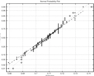
Figure 2 clearly illustrates the point in not over-dimensioning the particle filter. Here approximate MLEs of θ were computed from 50 samples of sizen= 1,000, using particle filters of sizes N = 300 andN = 1,500 respectively and with a five times denser grid in the latter case. The sample standard deviation of the 50 estimates so obtained was 0.013 and 0.012 respectively. Increasing N (and decreasing ∆) even further would decrease this variability only marginally, as the variation in the estimates is then totally dominated by the sample variation intrinsic to the maximum likelihood estimator itself (which decreases only withn). Thus, for a fixed sample size n it is sensible to choose N large enough that the variability of the parameter estimate due to the particle filter variation is smaller than the variability of the maximum likelihood estimator itself, while choosing N much larger is only cost ineffective. Figure 2 also shows that the approximate MLEs are approximately normal. Such an asymptotic result can indeed be verified, provided Nn increases faster than
what is required for consistency; see [4] for details.
References
0 0.1 0.2 0.3 0.4 0.5 0.6 0.7 0.8 0.9 1 −250
−200 −150 −100 −50 0 50 100
Theta
loglikelihood
1 2 3 0.64
0.66 0.68 0.7 0.72 0.74 0.76
Estimates
Figure 1. Left plot: Likelihood approximation based on a sample of sizen= 100 and particle
filter of sizeN = 110. Right plot: Box-plots of approximate MLEs computed from 30 samples of sizes n = 100, 1,000 and 2,000 respectively (left to right), with corresponding ∆n = 0.02,
0.0063 and 0.0045 andMn= 110, 385 and 560 respectively.
0.68 0.69 0.7 0.71 0.72 0.73 0.74 0.01
0.02 0.05 0.10 0.25 0.50 0.75 0.90 0.95 0.98 0.99
Estimates
Probability
Normal Probability Plot
Figure 2. Normal probability plots of approximate MLEs computed from 50 samples of size
n= 1,000 and particle filter sizesN = 300 (+) andN = 1,5000 (◦). I addition, the grid is five
times denser forN = 1,500.
[2] R. Douc, ´E. Moulines and T. Ryd´en, Asymptotic properties of the maximum likelihood estimator in autoregressive models with Markov regime,Ann. Statist.,32, 2002, pp. 2254–2304.
[3] A. Doucet, N. de Freitas and N. Gordon,An Introduction to Sequential Monte Carlo Methods, Springer, New York, 2001. [4] J. Olsson and T. Ryd´en, Asymptotic properties of the bootstrap particle filter maximum likelihood estimator for state-space
models. Preprint, Centre for Mathematical Sciences, Lund University, 2006.
[5] M.K. Pitt, Smooth particle filters for likelihood evaluation and maximisation. Preprint, Department of Economics, University of Warwick, 2002.