Cardiovascular Modeling With Adapted Parametric Inference

(1)

Muhammad DAUHOO, Laurent DUMAS, Pierre GABRIEL and Pauline LAFITTE

CARDIOVASCULAR MODELING WITH ADAPTED PARAMETRIC

INFERENCE

Didier Lucor & Olivier P. Le Maˆıtre

1

Abstract. Computational modeling of the cardiovascular system, promoted by the advance of fluid-structure interaction numerical methods, has made great progress towards the development of patient-specific numerical aids to diagnosis, risk prediction, intervention and clinical treatment. Nevertheless, the reliability of these models is inevitably impacted by rough modeling assumptions. A strong in-tegration of patient-specific data into numerical modeling is therefore needed in order to improve the accuracy of the predictions through the calibration of important physiological parameters. The Bayesian statistical framework to inverse problems is a powerful approach that relies on posterior sampling techniques, such as Markov chain Monte Carlo algorithms. The generation of samples re-quires many evaluations of the cardiovascular parameter-to-observable model. In practice, the use of a full cardiovascular numerical model is prohibitively expensive and a computational strategy based on approximations of the system response, or surrogate models, is needed to perform the data as-similation. As the support of the parameters distribution typically concentrates on a small fraction of the initial prior distribution, a worthy improvement consists in gradually adapting the surrogate model to minimize the approximation error for parameter values corresponding to high posterior den-sity. We introduce a novel numerical pathway to construct a series of polynomial surrogate models, by regression, using samples drawn from a sequence of distributions likely to converge to the posterior distribution. The approach yields substantial gains in efficiency and accuracy over direct prior-based surrogate models, as demonstrated via application to pulse wave velocities identification in a human lower limb arterial network.

1_{LIMSI, CNRS, Universit´}_{e Paris-Saclay, Campus universitaire bˆ}_{at 508, Rue John von Neumann, F-91405 Orsay cedex, France}

c

EDP Sciences, SMAI 2018

(2)

Résumé. En s’appuyant notamment sur les progrès réalisés dans le domaine des méthodes numériques pour l’interaction fluide-structure, la modélisation du système cardiovasculaire progresse fortement. Elle est aujourd’hui en passe de proposer des outils numériques personnalisés pour l’aide au diag-nostique, à la prédiction des risques, à l’intervention et au traitement clinique. Cependant la fia-bilité des simulations est inévitablement impactée par les approximations liées à une modélisation encore trop grossière ou partielle. L’intégration directe de données spécifiques au patient est donc souhaitable à l’amélioration de la précision des prédictions par le biais de l’inférence des paramètres physiologiques importants. Le cadre statistique du formalisme bayesien se prête naturellement à la resolution des problèmes inverses. Il s’appuie sur des techniques d’échantillonnagesa posteriori, telles que les méthodes de Monte Carlo par chaines de Markov. La génération de la chaine requiert de mul-tiples évaluations du modèle cardiovasculaire reliant les paramètres aux l’observables. En pratique, le recourt à un modèle cardiovasculaire complet reste trop couteux. Dans ce cas, le choix d’une stratégie de calcul reposant sur des approximations par un modèle de substitution de la réponse du système rend l’assimilation des données plus abordable. De plus, comme le support de la distribution des paramètres

a posterioritend à se concentrer sur une petite portion de la distribution a priori, une amélioration possible consiste à graduellement adapter le modèle de substitution de manière à minimiser l’erreur d’approximation pour les valeurs des paramètres ayant les plus grandes densitéa posteriori. Nous pro-posons une nouvelle approche numérique générant une suite d’approximations polynomiales du modèle, construite par régression à partir d’échantillons tirés aléatoirement selon une séquence de distributions convergeant vers la distributiona posteriori. Cette approche permet d’obtenir un gain numérique sub-stantiel en termes d’efficacité et de précision par rapport à une approximation polynomiale directement basée sur un échantillonnage selon la distributiona priorides paramètres. La méthode est appliquée au cas de l’assimilation de données d’un modèle hémodynamique humain de la propagation d’ondes de pouls dans le réseau artériel du membre inférieur.

Introduction

Inverse problems, encountered in the parametric identification, data assimilation or shape optimization are ubiquitous in life sciences and related interdisciplinary fields such as biomedical, biomechanics and bioengineer-ing applications. Bebioengineer-ing generally ill-posed, inverse identification often entails very large computational efforts as it requires to iteratively solve the equations characterizing the biological system (i.e. the forward problem) numerous times; the idea behind the process being to adjust some parameters in order to lower the discrepancy between the numerical prediction and some indirect clinical observations of the system. The computational burden of repeatedly solving the forward problem in order to get some outputs of interest is further ampli-fied because the model (e.g. patient-specific cardiovascular model) is often nonlinear and brings in unknown high-dimensional parameter spaces, and potentially large but noisy datasets. Model inversion in the presence of measurement errors must typically take advantage of some – type of regularization (e.g., Tikhonov regular-ization) in order to recover the existence and uniqueness of solutions or – robust optimization method [13]. A potentially more natural setting is the Bayesian statistics.

(3)

The accuracy of patient-specific cardiovascular simulation tools together with medical images and segmentation algorithms, has significantly increased in recent years, allowing for tremendous progress in the understanding and treatment of various medical conditions. One example of such achievements is the simulation of the full-scale fluid-structure interaction between the blood flow and the arterial walls of the systemic circulation network, thanks to the coupling of Navier-Stokes equations with elastic parietal models [49]. Nevertheless, reliability and sensitivity of this type of numerical predictions with respect to the model bio-physiological and biomechanical parametric uncertainties and errors are seldom reported. There exists for instance numerous uncertainties related to geometry (e.g., arterial wall thickness, lumen diameter in the case of stenosis model, lesion length), material properties (e.g., permeability, elasticity, compliance or Young’s modulus), blood rheology/viscosity, micro-vasculature peripheral resistance (e.g., the boundary conditions), etc. . . associated with cardiovascular simulations. When available, patient-specific data are often scarce and indirect observations of the quantity of interest (the model parameters) and are altered by measurements noise and/or averaging acquisition procedures (e.g., clinical and medical imaging). Otherwise, population-averaged values are commonly used in place of patient-specific data. In addition, accurate full-scale direct numerical simulations remain generally out of reach and are not of effective use in support to the clinician’s diagnostics and interventions. It is then a common usage to rely on reduced-order approximations (ROM), which are computationally more efficient but also more prone to model errors. After parametric calibration, the carefully crafted low-order model requires validation. In the case of vascular hemodynamics simulations, some exhaustive comparison between 1D and 3D hemodynamics formulations have for instance been published, e.g. [8, 30]. Several studies have shown the ability of the 1D formulation to capture the main features of pressure, flow and area waveforms in large human arteries usingin vivomeasurements [9, 31, 48], or in vitro experiments or 3D numerical data [8, 30]. Nevertheless, deterministic ROM constructed with optimized parameters value thanks to in vivo measurements or 3D numerical data often have limited value in predicting unobserved scenarios. Moreover, they do not provide an easy access to global parametric sensitivity analyses, that are essential to guide the modeling effort. Several works, e.g., [10, 12, 36–38], have demonstrated the interest of incorporating generic inter– and intra–patient variability in the form of uncertainty in the modeling of the cardiovascular system, since many aleatory and epistemic uncertainties remain due to its complexity, diversity and multiscale nature. These studies have shown how to propagate parametric uncertainties into the model in order to determine confidence intervals and statistics on the simulation predictions.

(4)

full FM is required.

The proposed inverse modeling approach focuses on the efficient characterization of sensitive reduced-order model parameters based on clinical data. In addition to the obvious asset of uncertainty reduction, thanks to the calibration, the stochastic modeling provides patient-specific quantitative information about the confidence in simulation predictions of unobserved cardiovascular states and points to the most influential parameters, thanks to calibrated global sensitivity analysis.

1. Adaptive cardiovascular surrogate

1.1. Parametric Bayesian inference based on surrogate reduced-order models

Here, we introduce our notations and recall the basics of Bayesian inference for parameter identification. Then we show how the formulation may be loosened to speed up the inference. We consider a forward model that maps some unknown parameters θ consider random to some observations, or the quantities of interest,

z derived from the forward model solution y. The vector of random parameters to be inferred is written as

θ ≡ θ(ω) = (θ(1)_{, . . . , θ}(nθ)₎ ∈ I

θ ⊆Rnθ_{, The FM solution (considered discrete) is a} _n

θ−variate functional

the parameters, y :Iθ → Iy ⊆Rny_{, so that the predicted quantities of interest are also random functionals:}

z : Iy ⊆ Rny → Iz ⊆ Rnd_{. Denoting} _d ∈

Rnd _{the dataset of observations (or measurements), the Bayes’}

formula writes:

πpost(θ|d)∝π`(d|θ)πprior(θ), (1)

where prior information aboutθis encoded in the prior densityπprior(θ),π`(d|θ) is the likelihood function that

incorporates both the data and the forward model andπpost(θ|d) the sought parameters posterior density. The

likelihood results from the combination of the costly deterministic forward model M:Rnd _× Rnx _→

Rny_{, an}

observation operator: G:_Rny _→

Rnd _{and statistical models for measurement noise and model error. Assuming}

additive measurement noise, mutually independent from the parameters, we have:

d=z+ε=G(y) +ε=G(M(θ,x)) +ε, (2)

where the distribution πε of ε is prescribed. In this case, we will assume that the noise model involves no

hyperparameters, so the likelihood function becomes:

π`(d|θ) =πε(d− G(M(θ,x))). (3)

The likelihood function therefore contains a stochastic source term whose representation must encompass the response of the deterministic forward model over the support ofπprior(θ). In practice, no closed form analytical

expression exists. Posterior moments, expectations or maximuma posteriorivalues must be estimated via sam-pling methods such as MCMC, which require many evaluations ofM(θ,x) and can range from a few thousands to a few millions depending on the problem. One obvious way to accelerate this computation is to substitute a faster and cheaper reduced-order model (ROM)Mromto the full deterministic forward model. Here we refer to

numerical reductions with respect to the xquantity, which denotes the variables or parameters of the system whom quantified representation is known (e.g. spatial coordinates).

Previous works have relied on ROMs to solve more efficiently computational inverse problems, exploiting either the deterministic, the frequentist [20], or the Bayesian approach [16]. For instance, deterministic reductions can be introduced using a Proper Orthogonal Decomposition [41] or a Reduced Basis method [32], dimension reduction, simpler geometry, etc...). A complementary approach consists in introducing a stochastic approxi-mation that will alleviate the systematic sampling of the (costly) forward model, e.g. [29]. In our case, we build a stochastic approximation of the ROM, i.e. a surrogate model noted ˆMrom, this time approximated in terms

(5)

takes the following form:

ˆ

πpost(θ|d)∝πε

d− GMˆrom(θ,x)

πprior(θ). (4)

The surrogate model should approximate the quantity of interest as accurately as possible. Classically, it is constructed from a finite set of model predictions for selected parameter values in a “off-line” stage, and subsequently used “in-line” during the sampling stage. The construction and querying of the surrogate model should be computationally efficient with sufficient predictive capabilities. Different methods are available to construct such surrogate models; examples are Gaussian processes [33], support vector machines [43], stochastic interpolation [44], or stochastic spectral methods such as polynomial–based representations. The choice of the surrogate model should be made to guarantee the accuracy of the approximate posterior distribution incurring from the substitution of the model prediction in Equation (4). Previous works have shown that the approximate posterior distribution error (in Kullback-Liebler divergence norm) is bounded by the surrogate model error measured in the mean square sense induced by the prior measure [7, 29]. Therefore, polynomial chaos surrogate

models [17,25,50] are well suited as they indeed minimize the error normkz−zˆk`2(πprior)= Eπprior{(z−ˆz)

2_}12_.

In this paper we will focus also on the use of polynomial expansions, that are well-suited for smooth de-pendences, constructed by discrete least-squares type approach. The surrogate model then consists in a linear combination of prescribed multivariate polynomials inθ. We shall assume thatz(θ) is a second order random vector forθ∼πprior(θ); its polynomial surrogate will write:

G(y(θ)) =z(θ)≈zˆ(θ) = X

γ∈Λp

aγψγ(θ), (5)

whereaγ are the unknown expansion coefficients, Λp is an multi-index set (to be defined) for multi-indexγ=

(γ1, . . . , γnθ)∈N

nθ_{. The polynomial approximation space is}

PΛp≡span{ψγ |γ∈Λp}, where the multivariate

polynomials are often constructed as product of one uni-variate polynomials,ψγ(θ) =Q nθ

i=1ψ (i)

γi (θ

(i)_{), with}_ψ(i)

γi having degreeγi. We restrict ourselves to isotropic tensor-product spaces total degree (TD)pleading to ΛTDp =

{γ∈Nnθ _:_||_γ_||

1≤p}. We shall assume that these polynomials set forms a basis for any subsequent measures

associated to θ, in particular the successive approximations of the posterior density. For simplicity in the construction of the original polynomial basis, we assume prior independence of the prior parameters. Posterior parameters however may be dependent or at least correlated. In this latter case, a numerical conditioning of the parameters samples (e.g. Cholesky-type decomposition), mapping the parameters into centered and normalized uncorrelated coordinates will facilitate the polynomial regression.

1.2. Adaptive weighted regression construction

The construction of accurate polynomial surrogates of general functions over large (prior) supports remains very challenging and demanding. Moreover, it is very inefficient in the context of Bayesian inference when the data are informative, i.e. when the posterior density of the inferred parameters highly concentrates from the initial prior density. A more efficient and accurate approximation can be obtained by constructing a “posterior-adapted” surrogate model that would minimize the kz −ˆzk`2(πpost), that is the error norm induced by the posterior. A legitimate concern is the one of the construction of a surrogate in the important region of the posterior distribution before actually characterizing the posterior. As this measure is not known from start, we propose a sequential strategy where a sequence of surrogates ˆM(romk), fork= 1,2, . . ., is iteratively adapted until

convergence, on the basis of model evaluations drawn from a sequence of posterior measure approximations ˆ

π(_postk) (θ|d).

(6)

the total number N of discrete samples of the mapping needed to construct the surrogate model. Because the parametric inference is driven by random sampling, we choose to rely on iterated polynomial regressions over sets of randomly generated points. Moreover, we make the choice of numerically emphasizing the samples for which the current surrogate ˆz(k) predicts wellz. This is ensured by associating scalar weights ρj _>_{0 to the}

samples in the resolution of polynomial regression problem. In the following, we explain how the samples are incorporated, weighted and used in the construction of the surrogates.

Let us assume, for the sake of comprehension, that we dispose of a current surrogate polynomial model ˆM(romk)

at some step (k) of our sequential process. This surrogate, constructed on the basis of a set of previous weighted model simulations S(k)_{, is fast to evaluate and serves the purpose of the MCMC sampler that produces a new}

set of parameters drawn from ˆπ(postk) (θ|d) according to the Bayes’ rule of Equation (4). One may then consider

a few numbern(k)_{of well-mixed parameters samples}_θ(k),1≤j≤nk _{of this chain, and performs the corresponding}

simulations using the ROM FM to compute z(θ(k), j). For each sample, one can then quantify the current

surrogate error using a discrepancy measure ∆j =

G

Mrom(θ(k),j,·)

− GMˆ(romk)(θ(k),j,·)

. There exists

different ways of deriving sample weights from the discrepancy measure, but the main idea is to make it inversely proportional with some numerical bounding capability, i.e. ρj_∼ _max(_,_∆j₎−1

[23]. If allρj_{are large, it means}

that the surrogate is quite accurate in the sampled approximate posterior region, implying in turn that ˆπ_post(k) approximates wellπpost. On the contrary, whenρj is low, it indicates that the sampleθ(k),j is not a reliable

ob-servation point as it is drawn from an inaccurate posterior. The sample weight completes the obob-servation triplets constituting the set A(k)₌_{₍_zj_,_θj_{, ρ}j₎_}

j=1,2,...,n(k) of observations collected at iteration k. This set is added to the current setAof all observations collected so far: A={(zj_,_θj

, ρj₎_}

j∈J={1,2,...,n=1+2+...+n(k−1)₊_n(k)_}.

At this stage, a choice needs to be made in order to selectamong this growing database A, the subset of samples that will be used to construct the next polynomial surrogate Mˆ(romk+1) at step (k+ 1). Again, there

is no unique bandwidth selection choice, and one may only consider selecting among the more recently gen-erated samples, select samples with larger trust indexes across multiple previous iterations, . . . Irrespective of the selection strategy, let us denoteS(k+1)_{≡ {}₍_zj_,_θj

, ρj)}j∈J(k+1)_⊆J the selected subset of A. Depending on the number and quality of the samples inS(k+1)_{, the approximation space must be tailored. A simple option}

consists in relating the total orderpof the polynomial approximation to the number of elements inS(k+1)_.

In this work we used the following strategy. First, to construct the initial (k= 0) surrogate model we set p(0)= 1 and generaten0samplesθj drawn directly from the priorπprior(θ) to obtained the initial set of triplets

using arbitrarily ρj= 1. The size of the initial set is n0= 3×npol(p(0)) where npol(p) is the dimension of the

TD polynomial space at degree p. The whole set is used to compute the initial surrogate, S(0) ₌_A_{. Then,}

at each iteration (k), we generate nf ×npol(p(k)) new samples from the current surrogate posterior, for some

nf ≥1 integer. The polynomial degree of the next surrogate is selecting according to the rule

p(k+1)=

(

p(k)_{+ 1} _if_n

f×npol(p(k)+ 1)≤ |A|/2,

p(k) otherwise.

For the construction, we attempt to use asymptotically the last half of the collected samples in A using the definition J(k+1) ₌_{_n₋_max(_n/₂_{, n}

f ×npol(p(k+1)), . . . , n}. Here, we choose nf = 2 to ensure at least twice

as many samples as polynomial coefficients. The value of nf can be increased to improve the stability of the

regression in particular whenp(k+1)_{becomes large.}

The surrogate model ˆM(romk+1)is finally determined solving (component-wise) the following weighted least squared

(7)

For each component, cf. Equation (5), the new model at the next iteration ˆM(romk+1) is therefore obtained by

solving a weighted least squared residual minimization problem:

a(k+1)= argmin

b∈RP(k+1)

X

j∈J(k+1) ρj

zj− X

γ∈Λ

p(k+1)

bγψγ(θj)

2

. (6)

The surrogate model is then incrementally optimized to minimize the response error in the posterior norm. Ifz

presents sufficient regularity with respect to the parameters, one may expect fast convergence with a reasonably low polynomial degree. This translates into significant reductions in the number of FM evaluations. The convergence may be monitored numerically, for instance observing the samples weight distribution. Finally, the iterations are continued until convergence is reached or a maximum number of iterations (kmax) or simulations |A|> N is attained.

2. Pulse wave velocities identification in cardiovascular systemic arterial

networks

In the following, we propose to apply our technique to the characterization of a subject-specific hemodynamic model of the pulse wave propagation in a vascular network. Quantifying the relationship between the physical properties of the cardiovascular system and the shape of the arterial pulse wave is important because the latter carries valuable information for the diagnosis and treatment of cardiovascular diseases. The coupled interaction of the blood flow with the network of compliant arteries is a (nonlinear) fluid-structure interaction (FSI) problem with a closed distribution network, pulsatile fluid flow with complex internal dynamics and multiple reflections leading to relatively complicated pulse wave patterns [46].

2.1. Arterial stiffness

Cardiovascular diseases, such as atherosclerosis, aneurysm, and dissection all involve significant degener-ation of the arterial wall tissue, e.g., deposition of calcified materials, reduction in elastin content, plaque formation [45]. These degenerations induce changes in the arterial stiffness, i.e., the capability of the vessel to accommodate and damp the pressure waves generated by the sudden change in blood pressure due to the heart systolic contraction. Arterial stiffening plays a key role in the development of cardiovascular diseases. Even if the exact mechanism by which it leads to increase in pulse pressure and systolic hypertension is still a controversial topic [34], it remains a valid predictor of cardiovascular morbidity and mortality. The problem is those stiffness properties of the aortic walls are not well known and subject to large (spatial) variabilities among individuals [35]. In fact, pulse wave velocities not only fluctuate during a cardiac cycle but also vary along the arterial tree due to the natural stiffening of the arterial walls toward distal locations. Arterial stiffness is hard to measure in vivo [47] and require numerical substitutes [1]. Common medical practice is to infer it from an indirect measurement of pressure (averaged) pulse wave velocity in the large vessels of the arterial tree – carotid-femoral or brachial-ankle assessments are common – thanks to medical imaging (Doppler Ultrasound, MRI, CTComputed Tomography) and the Moens-Korteweg equation [22]. For instance, the ankle-brachial arterial pressures index which reflects peripheral arterial obstruction due to atherosclerosis, is an established vascular marker for the diagnosis of peripheral arterial disease which affects more than 20% of the elderly pop-ulation. In this case, accurate modeling of the arterial pulse wave velocities in the limbs are critical to assessing the revascularization of the lower extremities and its impact on a major cardiovascular risk [18].

(8)

and physical constraints among parameters. Other studies have considered the assimilation of patient-specific clinical geometrical or functional data/measurements together with the use of a reduced-order model of the arterial circulation by relying on a deterministic or statistical formulation [3–6, 11, 13, 26]. When measurement error is included in the observations and uncertainty considered in the forward model describing the effect of the sought-after parameters onto the outputs, it results in a stochastic inverse problem whose solution is a probabilistic description of the parameters [3], in contrast with a point-wise estimate as in inverse problems. We propose to apply our approach to the calibration of an arterial hemodynamic model. We treat pulse wave velocities and arterial lumen area of the arteries at rest as piecewise-constant but unknown quantities mod-eleda priorias independent random variables (one for each artery component considered among {Ai}i=1...d=7

arteries). With the help of a simplified hemodynamic model together with patient-specific non-invasive local measurements of the vessel motion and blood flow velocity, we then apply our iterative approach in a Bayesian framework in order to efficiently calibrate these pulse wave velocities.

2.2. Reduced-order model of the distributed blood circulation

2.2.1. Governing equations

We consider a portion of the systemic arterial tree containing a finite number of arteries: we have a network of thin, deformable, and axisymmetric arterial segments filled with blood, taken as an incompressible Newtonian fluid [40]. The formulation, for each arterial segment, based on the conservation of mass and momentum laws and on Young-Laplace equation, is:

∂A ∂t +

∂Au

∂x = 0

∂u ∂t +u

∂u

∂x = −

1 ρ

∂p ∂x+

f ρ A

p = p0+β √

A−pA0

, (7)

where t denotes time, x∈ D is the axial coordinate along the arterial centerline, A(x, t) is the circular cross-sectional area of the lumen, u(x, t) and p(x, t) are average velocity and internal pressure, respectively, ρ is blood density. The term f is the friction force per unit length and is related to the velocity profile through f = −2µπ α

α−1u, where µ is blood dynamic viscosity and α ∈ [0,1[ is a correction factor accounting for the nonlinear integration of radial velocities in each cross-section [42]. The underscript 0 denotes quantities

at rest. The β parameter is a measure of the arterial wall stiffness related to its mechanical behavior: β =

√

π h0E/(1−ν2)A0, whereh0is the reference arterial wall thickness,E is the Young’s modulus andν= 1/2 is

the constant Poisson’s ratio. It is also related to the pulse wave velocitycthrough the following relation:

β = 2ρ c

2₍_{x, t}₎

p

A(x, t)= 2ρ c2

0 √

A0

. (8)

Note thatcandc0increase with increasing elastic modulus and wall thickness, and decreasing luminal area.

At some point in the following, due to the lack of knowledge of the pulse wave velocity at rest c0, it will be

modeled as a random quantity which implicitly denotes the uncertainty in Young’s modulus. We refer the reader to [15] for more details about the mathematical form of this system of equations.

2.2.2. Numerical solver

(9)

Detailed mathematical formulation and analysis about the hyperbolic system and the numerical scheme may be found elsewhere, e.g. [9].

We use an explicit second-order Adams-Bashforth scheme with a time step dictated by the CFL condition [21]. In the case of polynomial approximation of order p= 4 within each cell, pulse pressure convergence is reached for an average mesh resolution of 20 cells per unit meter. Dirichlet-type time-dependent boundary conditions at the inlet of the domain are imposed thanks to subject-specific echo-tracking clinical data. At each exit of the simulated arterial tree, a simple terminal reflection is imposed via a scalar coefficientR∈[0,1] that relates the backward to the forward characteristic information. It enables the simulation of reflected waves induced by the resistances of the missing peripheral arterioles and capillaries. This coefficient may be interpreted as an avatar of a lumped parameter model made of a single resistance [2, 13].

3. Numerical results

3

7 5

Deep femoral

Posterior tibial Descending

genicular

Femoral

Poplital

Anterior tibial

2

4

6 1 Iliac

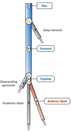
Figure 1. Network of the seven main human lower limb arteries. Resistance symbols represent

partially reflecting outflow boundary conditions. Some medical imaging data relative to local temporal evolutions of cross-sectional area and blood flow velocity are available in the arteries in blue; only flow velocity data are available for the artery in red; nothing is measured in the arteries in grey color.

In the following, we are interested in a subject-specific data assimilation on an arterial human left lower limb model. Here we consider the same seven-artery simple network model described in details in reference [13], where – only the largest arteries are retained and physiological properties at rest are considered piecewise constant, see Figure (1) and for some of which – we hold some medical imaging data. The non-invasive measurements are collected on the male subject thanks to ultrasound echo-tracking technique [14]. The data are cross-sectional lumen areaA(xcenter, t) changes measured at the approximatecenter of the iliac, femoral and poplital arteries {Ai}i=1,2,4, and blood velocity changes u(xcenter, t) measured at the same locations and at the center of the

anterior tibial artery {A6} as well, see Figures (1,5). These data are collected non-simultaneously for the

(10)

beat) during the clinical examination. In order to reduce these uncertainties and also to make the application more challenging, we condense the temporal information into scalar quantities. Contrarily to the study of El Bouti [13], where entire time signals were put to use, here the data are utilized in the form of scalar relative arterial changes measured over time: d≡ {dl}l=1:nd ∈R

nd=7 _with:

dl≡

φ{Ai(l)}(xcenter, t

sys₎₋_φ

{Ai(l)}(xcenter, t

dia₎_/φ

{Ai(l)}(xcenter, t

dia₎

, (9)

where φ{Ai(l)} is thel

−th _{measured quantity at the center of the artery}_{_A

i(l)}, and tsys andtdia relate to the

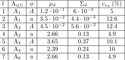
cardiac systolic (diastolic) time at which the measured quantity reaches its maximum (minimum) respectively. For the data we have access to, the measured quantity is either the lumen area or the blood flow velocity. Due to the lack of information, measurements statistical description is evaluated from the collected time signals and modeled as=N(µd,Σd). In particular, Σdis directly approximated from the signals temporal deviation

which is a very crude assumption that does not account for instance for measurements errors due to approximate spatial acquisition sites and non-simultaneous acquisition times. The statistical description is summarized in Table 3. The chosen values are such that the coefficient of variations of these measurements exhibit a 40% dispersion.

l Ai(l) φ µd Σd cvd (%)

1 A1 A 1.2·10−1 6·10−3 5

2 A1 u 3.5·10−2 4.4·10−3 12.6

3 A2 A 4.5·10−2 5.6·10−3 12.4

4 A2 u 2.66 0.13 4.9

5 A4 A 3.65 0.37 10.1

6 A4 u 2.39 0.24 10

7 A6 u 2.66 0.13 4.9

Table 1. Measurements dataset description and statistics (means, standard deviations and

coefficient of variations), cf. Eq. (9).

The main parameters to be inferred are the pulse wave velocities at restc0∈Rd=7in all arteries{Ai}i=1,...,d=7

of the network. Meanwhile, we also infer the resistance parameters at each outflow boundary condition, i.e.

R∈Rd=4in arteries{Ai}i=3,5,6,7and the lumen cross-section of the arteries at rest that have not been measured,

i.e. A0∈Rd=4 in arteries{Ai}i=3,5,6,7. All the parameters, θ∈Rd=15, are expresseda priori as independent normal random variables with p(θ)∼ N(µθ,Σθ). Mean values µθ and standard deviation Σθare chosen from

the literature [39], and correspond to coefficient of variations of the order of cvθ ∼ 15%. In practice, these

statistics insure positivity and satisfy the hyperbolicity condition of the system [51] almost surely.

The iterative surrogate model of the system response is adaptively constructed based on the following numerical tools: – a deterministic parallelized DG 1D fluid-structure interaction hemodynamic solver (here with a typical resolution: h∼0.2 cell/cm; and a Legendre polynomial approximation basis of orderp= 4 in each mesh cell); – an automated data samples selector and preconditioner; – a set of orthonormal polynomial (here Hermite) libraries of arbitrary degree p and cardinality npol (here relying on tensor-products constructed to satisfy a total degreeexpansion) and – a weighted least-squarew−LS solver; the posterior sampling of the parameters is handled thanks to parallel MCMC chains (Metropolis-Hastings scheme) of 3.2·105samples.

(11)

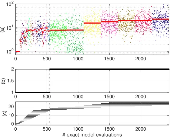
of the adaptive surrogate construction for N = 25001 _and _p(0) _{= 1, reporting the evolution of the samples}

trust-index value (colored dots) and their average (red solid line) over the new data completing at each iteration (k) the total data setA. The results are reported as a function of the cumulated number of exact model solves; also reported is the evolution of the surrogate model order p(k) and the corresponding set of selected J(k)

samples in Figures 2–(b-c). We see from the plot that the averaged trust-index globally increases, denoting the progressive improvement of the surrogate. Vertical black dotted lines materialize the points at which the surrogate order is automatically incremented. We notice patent increases when the surrogate order is augmented. Posterior statistics convergence (not displayed here) show that mean values are nicely calibrated and reach asymptotically statistically stable values after about ∼500 model evaluations. Concerning the std results, the data are informative enough so that the uncertainty ranges are often reduced.

0 500 1000 1500 2000

100 101 102

(a)

0 500 1000 1500 2000

1 1.5 2

(b)

0 500 1000 1500 2000

# exact model evaluations

0 10 20

(c)

Figure 2. Evolutions of the sample trust-indices (colored dots) and their averages (solid red

lines) (a), selected polynomial orderp(k)_{(b) and corresponding selected}_J(k)_{samples (c) used}

to build the successive surrogates vs. the total number of hemodynamic model evaluations.

Figure 3 presents one- and (joint) two-dimensional marginal distributions of the pulse wave velocities at restc0 obtained from kernel density estimates at the final iteration of the numerical approximation procedure.

Other inferred parameters distributions are not represented as they are less influent. Globally we can say that the measurements in {A2,4,6} arteries are informative enough in the sense that the stiffness uncertainty

of the material system is lowered except in distal arteries {A3,5,7}. It is particularly true for the top {A1}

artery. Located upstream of the network and contiguous of the deterministic inflow boundary condition, the system response in this artery is not prone to large uncertainties. Feeding on the downstream measurements, the arterial stiffness of this vessel is therefore sharply calibrated. This directly benefits the calibration of the connected downstream main arteries, in particular, {A2,4,6}. In fact, we observe very noticeable correlations

between the stiffness of arteries{A1,2}, {A1,4} and also{A2,4}. This makes sense due to the topology of the

network, see Figure 1. We also notice that joint measures between the stiffness of {A6} and each of {A1,2,4}

get nicely informed from the bayesian updating. The stiffness of artery {A7} is somewhat updated but one

1_{This computational budget was chosen to match the total number of solver evaluations of the optimization algorithm in}

(12)

Nominal CMA-ES optimization Bayesian inference (MAP) Artery # A0 (cm2) c0 (m/s) R A0 (cm2) c0 (m/s) R A0(cm2) c0(m/s) R

1(A,u) _0.53 _7.20 _- _0.53 _4.99 _- _0.53 _5.35

-2(A,u) 0.47 9.15 - 0.47 11.96 - 0.47 11.28

-3 0.3 8.32 0.65 0.27 7.39 0.48 0.29 8.86 0.65

4(A,u) _0.4 _9.50 _- _0.40 _10.51 _- _0.40 _10.9

-5 0.3 9.95 0.65 0.32 9.93 0.42 0.33 8.7 0.52

6(u) _0.2 _11.12 _0.65 _0.23 _11.61 _0.95 _0.20 _8.97 _0.75

7 0.2 14.03 0.65 0.22 9.91 0.73 0.20 13.85 0.67

Table 2. Nominal and calibrated hemodynamic model parameters values estimated from

op-timization methods [13] and statistical inference (bold figures are obtained from measurements and are fixed). Calibrated pulse wave velocities relative error between genetic optimization and Bayesian inference is about 15% in average;c0values represented in italic exceed this threshold.

should be cautious as previous results have shown that the surrogate model might not be fully stabilized for this vessel. Finally, there still exists significant residual uncertainty in the arterial stiffness of {A3} and{A7}.

Joint marginal distributions between distal outflow arteries without measurements (i.e. {A3,5,7}) do not get

informed and remain very similar to their prior distributions. We have noticed that the final level of uncertainty

0 10 20 0 1 2

0 10 20 0 0.5

0 10 20 0 0.2 0.4

0 10 20 0 0.5

0 10 20 0 0.2 0.4

0 20 40 0 0.2 0.4

Figure 3. One- and two-dimensional pulse wave velocitiesc0posterior (colored lines) vs. prior

(gray lines) marginal distributions. Posterior distributions are estimated from the final iteration of the posterior-adapted surrogate method proposed. Results from artery {A1} to {A7} are

ordered from top to bottom row and from left to right column. Results for arteries sharing a bifurcation node are framed with an axis box.

is considerably reduced for some of the parameters. In particular, the posterior distributions are sometimes far distant from the prior measures, e.g. ˆπ(kfinal)

post (c01, c02) or ˆπ

(kfinal)

(13)

of interest. Once the right region is reached, more available samples render possible the construction of a higher-order polynomial approximation of the response, which makes the surrogate-based posterior sampling more efficient.

The Bayesian formulation also gives access to a valuable point-wise estimate of the inferred parameters: the

2 4 6 8 10 12 14

c 0

1 0

0.2 0.4 0.6 0.8 1 1.2

2 4 6 8 10 12 14 16

c 0

2 0

0.1 0.2 0.3 0.4 0.5 0.6 0.7 0.8

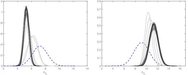
Figure 4. Pulse wave velocitiesc0marginal distribution in the iliac (left) and femoral (right)

arteries. Dashed lines represent prior distributions. Gradual color shading illustrates the se-quential progression of posterior distributions toward convergence (from light to dark colors) in regions of low prior probability.

maximum a posteriori probability (MAP) estimate that is defined as the mode of the posterior distribution: ˆ

θMAP = argmaxθπˆpost(θ|d). In the following, we compare the results of the numerical model relying on the

MAP hemodynamic parameters with those calibrated with a different approach. Another interesting subsequent study would have been to perform an uncertainty quantification of the effect of the entire probabilistic description of the calibrated parameters onto the quantity of interest.

Finally, the adaptively weighted regression approach yielded substantial gains in efficiency and accuracy over methods using direct prior-based surrogate models. A practical comparison – not presented here – was made for a similar but simpler version of the lower limb system introduced previously, i.e. with only seven stiffness parameters to calibrate. Our adaptive surrogate model approach was about one order of magnitude more efficient in terms of number of calls to the deterministic solver compared to a calibration based on a global surrogate model constructed over the prior parametric domain from a Gauss-Hermite Smolyak-designed sparse grid.

3.1. Comparison with an evolutionary optimization approach

(14)

about phasing nor timing.

Finally, figure 5 compares the predictions based on the nominal and MAP parameters values with the subject-specific measurements. The improvement is patent with the calibrated parameters, except for the cross-sectional lumen area in the iliac and the tibial arteries. Indeed, in the first case, the imposition of the upstream boundary condition data in the form of the measured area, is sufficient to drive the dilatation of the iliac artery to the right profile, even with parameters nominal values. In the second case, the measurements are not informative enough to induce real changes in the lumen area profile of the tibial arteries. Predictions obtained from the optimization procedure, see Fig. 9 in [13] look very similar, in particular for the first, second and third generations of arteries of the bifurcating network.

0 0.5 5 5.5 6 6.5 A (m 2 ) 10-5 0 0.5 4.6 4.8 5 5.2 10-5 0 0.5 3.8 4 4.2 4.4 10-5 0 0.5 1.8 2 2.2 2.4 10-5 0 0.5 (a) -0.5 0 0.5 u (m/s) 0 0.5 (b) -0.5 0 0.5 0 0.5 (c) -0.2 0 0.2 0.4 0 0.5 (d) -0.2 0 0.2 0.4 measured nominal MAP

Figure 5. Comparison between measured, nominal and calibrated cross-sectional lumen area

(top row) and blood flow velocity (bottom row) waveforms at the midpoint of some of arteries of the lower limb network in Figure 1, with (a): iliac, (b): femoral, (c): popliteal and (d): anterior tibial arteries.

4. _Conclusion

(15)

with the ones obtained using an alternative approach based on an evolutionary optimization algorithm. In addition, our approach provides richer information in the form of a complete statistical characterization of the inferred parameters. This result is remarkable considering that: a) the deterministic reduced-order model is quite simplified compared to a more sophisticated full three-dimensional fluid-structure interaction model, both in terms of network geometry, scales, and numerical modeling assumptions; b) the subject-specific real clinical data of different nature are scarce and incomplete; and c) the computational budget is relatively modest regarding the high-dimensional parametric space to explore.

The first author is greatly thankful to Prof. L. Dumas from the Laboratoire de Math´ematiques de Versailles, UVSQ, CNRS, Universit´e Paris-Saclay, France, for the organization and the invitation at the “Mathematical models in biology and medecine” school in Mauritius in 2016. The authors are also thankful to Prof. P. Boutouyrie from the Paris-Cardiovascular research Center (PARCC) at the Georges-Pompidou European Hospital (HEGP), Paris, France, for providing the echo-tracking measurements.

References

[1] J. Alastruey,Numerical assessment of time-domain methods for the estimation of local arterial pulse wave speed, Journal of Biomechanics, 44 (2011), pp. 885–891.

[2] J. Alastruey, K. H. Parker, J. Peiro, and S. J. Sherwin,Lumped parameter outflow models for 1-d blood flow simulations: Effect on pulse waves and parameter estimation, Communications in Computational Physics, 4 (2008), pp. 317–336. [3] F. Auricchio, M. Conti, A. Ferrara, and E. Lanzarone, A clinically applicable stochastic approach for noninvasive

estimation of aortic stiffness using computed tomography data, IEEE Trans Biomed Eng, 62 (2015), pp. 176–187.

[4] L. Bertagna, M. D’Elia, M. Perego, and A. Veneziani,Data Assimilation in Cardiovascular Fluid–Structure Interaction Problems: An Introduction, Springer Basel, Basel, 2014, pp. 395–481.

[5] C. Bertoglio, D. Barber, N. Gaddum, I. Valverde, M. Rutten, P. Beerbaum, P. Moireau, R. Hose, and J.-F. Gerbeau, Identification of artery wall stiffness: In vitro validation and in vivo results of a data assimilation procedure applied to a 3d fluid–structure interaction model, Journal of Biomechanics, 47 (2014), pp. 1027 – 1034.

[6] J. Biehler, S. Kehl, M. W. Gee, F. Schmies, J. Pelisek, A. Maier, C. Reeps, H.-H. Eckstein, and W. A. Wall, Probabilistic noninvasive prediction of wall properties of abdominal aortic aneurysms using bayesian regression, Biomechanics and Modeling in Mechanobiology, 16 (2017), pp. 45–61.

[7] A. Birolleau, G. Po¨ette, and D. Lucor,Adaptive Bayesian inference for discontinuous inverse problems, application to hyperbolic conservation laws, Communications in Computational Physics, 16 (2014), pp. 1–34.

[8] E. Boileau, P. Nithiarasu, P. J. Blanco, L. O. Muller, F. E. Fossan, L. R. Hellevik, W. P. Donders, W. Huberts, M. Willemet, and J. Alastruey,A benchmark study of numerical schemes for one-dimensional arterial blood flow modelling, International Journal for Numerical Methods in Biomedical Engineering, 31, p. e02732.

[9] E. Bollache, N. Kachenoura, A. Redheuil, F. Frouin, E. Mousseaux, P. Recho, and D. Lucor,Descending aorta subject-specific one-dimensional model validated againstin vivodata, Journal of Biomechanics, 47 (2014), pp. 424–431. [10] A. Brault, L. Dumas, and D. Lucor,Uncertainty quantification of inflow boundary condition and proximal arterial

stiffness-coupled effect on pulse wave propagation in a vascular network, International Journal for Numerical Methods in Biomedical Engineering, (2017). e2859 cnm.2859.

[11] A. Caiazzo, F. Caforio, G. Montecinos, L. O. Muller, P. J. Blanco, and E. F. Toro,Assessment of reduced-order unscented kalman filter for parameter identification in 1-dimensional blood flow models using experimental data, International Journal for Numerical Methods in Biomedical Engineering, (2017), pp. n/a–n/a. cnm.2843.

[12] P. Chen, A. Quarteroni, and G. Rozza,Simulation-based uncertainty quantification of human arterial network hemody-namics, International Journal for Numerical Methods in Biomedical Engineering, 29 (2013), pp. 698–721.

[13] L. Dumas, T. El Bouti, and D. Lucor, A robust and subject-specific hemodynamic model of the lower limb based on non-invasive arterial measurements, J. Biomech. Eng., doi: 10.1115/1.4034833 (2016).

[14] T. El Bouti, L. Dumas, and D. Lucor, Blood flow modeling and application to non-invasive determination of arterial stiffness, in ECCOMAS CFD 2014 Proceedings of the VI European Conference on Computational Fluid Dynamics, A. Huerta, ed., Barcelona, Spain, July 2014.

[15] L. Formaggia, D. Lamponi, and A. Quarteroni,One-dimensional models for blood flow in arteries, Journal of Engineering Mathematics, (2003), pp. 251–276.

(16)

[18] G. Giugliano, L. D. Serafino, C. Perrino, V. Schiano, E. Laurenzano, S. Cassese, M. D. Laurentis, G. G. Schi-attarella, L. Brevetti, A. Sannino, G. Gargiulo, A. Franzone, C. Indolfi, F. Piscione, B. Trimarco, and G. Espos-ito,Effects of successful percutaneous lower extremity revascularization on cardiovascular outcome in patients with peripheral arterial disease, International Journal of Cardiology, 167 (2013), pp. 2566 – 2571.

[19] N. Hansen and A. Ostermeier,Completely derandomized self-adaptation, evolution strategies, Evolutionary Computation, 9 (2001), pp. p.159–195.

[20] D. Huynh, D. Knezevic, and A. Patera,Certified reduced basis model validation: A frequentistic uncertainty framework, Computer Methods in Applied Mechanics and Engineering, 201–204 (2012), pp. 13 – 24.

[21] G. E. Karniadakis and S. Sherwin, Spectral/hp element methods for CFD, Oxford University Press, New York, second edition (2005).

[22] D. Korteweg,Uber die Fortpflanzungsgeschwindigkeit des Schalles in elastischen R¨¨ ohern, Ann. Phys. Chem. (NS), 5 (1878), pp. 525–527.

[23] J. V. Langenhove, D. Lucor, and A. Belme,Robust uncertainty quantification using preconditioned least-squares polynomial approximations with`1-regularization, International Journal for Uncertainty Quantification, 6 (2016), pp. 57–77.

[24] T. Lassila, A. Manzoni, A. Quarteroni, and G. Rozza,A reduced computational and geometrical framework for inverse problems in hemodynamics, International journal for numerical methods in biomedical engineering, 29 (2013), pp. 741–776. [25] O. P. Le Maˆıtre and O. M. Knio,Spectral Methods for Uncertainty Quantification with applications to Computational Fluid

Dynamics, Scientific Computation, Springer Netherlands, 2010.

[26] C. A. Leguy, E. M. Bosboom, H. Gelderblom, A. P. Hoeks, and F. N. van de Vosse,Estimation of distributed arterial mechanical properties using a wave propagation model in a reverse way, Med Eng Phys, 32 (2010), pp. 957–67.

[27] J. Li and Y. Marzouk,Adaptive construction of surrogates for the bayesian solution of inverse problems, SIAM J. Sci. Comp., 36 (2015), pp. A1163–A1186.

[28] D. Lombardi,Inverse problems in 1D hemodynamics on systemic networks: A sequential approach, International Journal for Numerical Methods in BioMedical Eng., 34 (2013).

[29] Y. Marzouk and D. Xiu,A stochastic collocation approach to bayesian inference in inverse problems, Comm. Comput. Phys., 6 (2009), pp. 826–847.

[30] X. N., A. J., and F. C.,A systematic comparison between 1-D and 3-D hemodynamics in compliant arterial models, Inter-national Journal of Numerical Methods in Biomedical Engineering, 30 (2014), pp. 204–231.

[31] M. S. Olufsen, C. S. Peskin, W. Y. Kim, E. M. Pedersen, A. Nadim, and J. Larsen,Numerical simulation and ex-perimental validation of blood flow in arteries with structured-tree outflow conditions, Annals of Biomedical Engineering, 28 (2000), pp. 1281–99.

[32] J. S. Peterson, The reduced basis method for incompressible viscous flow calculations, SIAM Journal on Scientific and Statistical Computing, 10 (1989), pp. 777–786.

[33] C. E. Rasmussen and C. K. I. Williams,Gaussian Processes for Machine Learning, The MIT Press, 2006.

[34] P. Reymond, N. Westerhof, and N. Stergiopulos,Systolic hypertension mechanisms: Effect of global and local proximal aorta stiffening on pulse pressure, Ann. Biomed. Eng., 40 (2012), pp. p.742–749.

[35] S. Roccabianca, C. Figueroa, G. Tellides, and J. Humphrey,Quantification of regional differences in aortic stiffness in the aging human, Journal of the mechanical behavior of biomedical materials, 29 (2014), p. 10.1016/j.jmbbm.2013.01.026. [36] S. Sankaran, L. Grady, and C. A. Taylor,Impact of geometric uncertainty on hemodynamic simulations using machine

learning, Computer Methods in Applied Mechanics and Engineering, 297 (2015), pp. 167 – 190.

[37] S. Sankaran and A. L. Marsden,A stochastic collocation method for uncertainty quantification and propagation in cardio-vascular simulations, Journal of Biomechanical Engineering, 133 (2011), pp. 1–12.

[38] D. E. Schiavazzi, G. Arbia, C. Baker, A. M. Hlavacek, T. Y. Hsia, A. L. Marsden, I. E. Vignon-Clementel, and T. M. of Congenital Hearts Alliance (MOCHA) Investigators,Uncertainty quantification in virtual surgery hemodynamics predictions for single ventricle palliation, International Journal for Numerical Methods in Biomedical Engineering, 32 (2016), pp. e02737–n/a. e02737 cnm.2737.

[39] S. J. Sherwin, L. Formaggia, and J. Peir´o,Computational modelling of 1D blood flow with variable mechanical properties, in ECCOMAS CFD, Swansea, UK, September 2001.

[40] S. J. Sherwin, L. Formaggia, J. Peiro, and V. Franke,Computational modelling of 1D blood flow with variable mechanical properties and its application to the simulation of wave propagation in the human arterial system, International Journal for Numerical Methods in Fluids, 43 (2003), pp. 673–700.

[41] L. Sirovich,Turbulence and the dynamics of coherent structures part i: Coherent structures, Quarterly of Applied Mathe-matics, 45 (1987), pp. 561–571.

[42] N. Smith, A. J. Pullan, and P. J. Hunter,An anatomically based model of coronary blood flow and myocardial mechanics, SIAM J. Appl. Math., 62 (2001).

[43] A. J. Smola and B. Sch¨olkopf,A tutorial on Support Vector Regression, Tech. Rep. TR-98-030, NeuroCOLT, 1998. [44] M. Tatang, W. Pan, R. Prinn, and G. McRae, An efficient method for parametric uncertainty analysis of numerical

(17)

[45] M. Thiriet,Biology and Mechanics of Blood Flows. Part II: Mechanics and Medical Aspects, CRM Series in Mathematical Physics, Springer, 2007.

[46] F. N. van de Vosse and N. Stergiopulos,Pulse wave propagation in the arterial tree, Annual Review of Fluid Mechanics, 43 (2011), pp. 467–499.

[47] J. Vappou, J. Luo, and E. E. Konofagou,Pulse wave imaging for noninvasive and quantitative measurement of arterial stiffness in vivo, American Journal of Hypertension, 23 (2010), pp. 393–398.

[48] M. Willemet, V. Lacroix, and E. Marchandise,Validation of a 1D patient-specific model of the arterial hemodynamics in bypassed lower-limbs: Simulations againstin vivomeasurements, Medical Engineering and Physics, 35, pp. 1573–1583. [49] N. Xiao, J. D. Humphrey, and C. A. Figueroa,Multi-scale computational model of three-dimensional hemodynamics within

a deformable full-body arterial network, Journal of Computational Physics, 244 (2013), pp. 22 – 40. Multi-scale Modeling and Simulation of Biological Systems.

[50] D. Xiu and G. Karniadakis,The Wiener-Askey polynomial chaos for stochastic differential equations, SIAM Journal on Scientific Computing, 24 (2002), pp. 619–644.