A Study on Properties of Dempster-Shafer Theory to
Probability Theory Transformations
A. Shahpari* and S. A. Seyedin**(C.A.)
Abstract: In this paper, five conditions that have been proposed by Cobb and Shenoy are studied for nine different mappings from the Dempster-Shafer theory to the probability theory. After comparing these mappings, one of the considerable results indicates that none of the mappings satisfies the condition of invariance with respect to the marginalization process. In more details, the main reason for this defect is that the classic projection process in DST loses some probabilistic information. For solving this problem, the modified pignistic probability and the modified normalized plausibility transformation which are invariance under marginalization are proposed. The two modified mappings are utilized in two ambiguity measures in Dempster-Shafer theory. Then, similar to the mutual information in the probability theory, these measures are used for computing the dependency of the variables of a social bliss problem on the person's happiness value.
Keywords: Ambiguity, Dempster-Shafer Theory, DST to PT Transformation, Invariance with Respect to the Marginalization Process, Normalized Plausibility Transformation, Pignistic Probability.
1 Introduction1
The Dempster-Shafer Theory (DST) and the Probability Theory (PT) are two theories that have been used for modeling uncertain data. In each theory, the combination and the marginalization rules are utilized for various applications. The main different of these two theories is that the Dempster-Shafer theory includes probability theory as well as set theory. In other words, in the Dempster-Shafer theory, the Basic Probability Assignment (BPA) is applied to assign masses to a subset of the frame of discernments while in the probability theory, the Probability Density Function (PDF) assigns values to the singleton members. The problems arise when we want to make a decision in DST. Therefore, the BPA in DST should be transformed to the probability density function in PT.
Some of these mappings are , , , , and that proposed by Sudeno [1], as defined by Cuzzolin [2], the pignistic probability ( as defined by Philippe Smets [3-6], and as proposed by Smarandache et al. [7]. Besides the issue of decision making, these mappings are utilized in the aggregate uncertainty measures for computing the amounts of information in DST.
Iranian Journal of Electrical & Electronic Engineering, 2015. Paper first received 03 Dec. 2013 and in revised form 18 Jan. 2015. * The Authors are with the Department of Electrical Engineering, Ferdowsi University of Mashhad, Mashhad 9177948974, Iran. E-mails: al_shahpari@yahoo.com, seyedin@um.ac.ir.
Smarandache et al. used the Probabilistic Information Content (PIC) as a measure of uncertainty for several probabilistic mappings from the DST to the PT. After comparing the mappings, they concluded that some mappings have conceptual problems and cannot produce acceptable results [7]. Klir et al. proposed AU as an aggregate uncertainty measure to compute the amounts of ambiguity in DST [8]. AU was defined based on another DST to PT mapping is denoted by . as it is defined by the optimization process of the algorithm 6.1 [9-12].
Jousselme et al. used the pignistic probability to measure ambiguity (AM) in Dempster-Shafer theory [13]. But, AM dose not satisfy the subadditivity condition which is one of the necessary properties of an aggregate uncertainty measure. The cause of this defect which was found by Klir in [14] was the dependency of the pignistic probability on the marginalization process.
Another application of these mappings is transforming a Dempster-Shafer network into a Bayesian network. In several articles, Cobb and Shenoy have compared two mappings, the pignistic probability and the normalized plausibility transformation [15-18]. They proposed five conditions should be satisfied by a DST to PT transformation. These conditions are: Invariance with respect to marginalization, Invariance with respect to combination, Idempotency, Unique most probable state, and Non-Unique most probable state.
The aim of this paper is to study the conditions mentioned by Cobb and Shenoy for nine mappings
namely, , , , , ,
, , , and . . Furthermore, some considerable results are obtained. Another important matter which was addressed here is the invariance with respect to marginalization property of two mappings, the pignistic probability and the normalized plausibility transformation. The key of the Invariance with respect to marginalization problem of and is in the projection and marginalization processes in DST. It can be shown that in the projection procedure, some probabilistic information is lost. If this data can be retained, the problem will be overcome. Based on this, a new set is presented which can store the probabilistic information lost in the projection process, and subsequently, the marginalization formula is slightly changed. Then, the modified pignistic probability and the modified normalized plausibility transformation are proposed that are invariant under the marginalization process.
The outline of this paper is as followings: In Section 2, we describe some necessary theoretical concepts. In Section 3, the nine mappings from DST to PT are represented and the Cobb and Shenoy’s requirements are investigated for these mappings. In Section 4, the invariance with respect to the marginalization property is descripted and the modified pignistic probability and the modified normalized plausibility transformation are proposed that are invariant under the marginalization process. In Section 5, these modified mapping are utilized in two new ambiguity measures and are used to compute the dependency of the variables of a social bliss problem to the person's happiness value. Finally, in Section 6, some concluding remarks are made.
2 Theoretical Background
In the probability theory, a PDF : 0,1
assigns values to , , … , (the state space of variable X), where 0, and ∑ : 1.
Definition 1. If and are the state spaces of variables and , then the joint state space is denoted
by and : 0,1 is the
corresponding joint PDF.
Marginalization in the probability theory involves addition over the state space of the variables being eliminated. Suppose is a joint PDF for , the
marginal PDF for is X ∑ , .
Combination in PT with Bayes’ rule involves “point wise” multiplication of probability density functions. Suppose is a PDF for and is a PDF for . Then, is a PDF for and defined as follows:
for each , where K is the normalization constant.
Dempster-Shafer theory is an imprecise probability theory in which a basic probability assignment (BPA) assigns values to the subsets of the state space [19, 20].
The function : 2 X 0,1 is a BPA on the power set
of , , … , , where 0, 0,
and ∑ ΩX 1. Any element in 2 X with a
non-zero BPA is called a focal element. Two other functions defined in DST are the belief function (
∑B and the plausibility function (
∑ B .
Topics such as joint state space, projection, and marginalization in DST are defined as follows:
Definition 2. If 2 X and 2 Y are the state spaces of
variables and with cardinalities 2| X| and 2| Y|, then
the joint state space is denoted by 2 XY and defined by
. Its cardinality is 2| XY|.
Example 1. If X , and Y , , are the state spaces of and , then the joint state space
in DST will be
2 (
, , , , , , , , , , , ),
and have 2| XY| 2 64 members. To put it simply,
we introduce the following notation:
Z , Z , Z , Z , Z , Z .
If and are the state spaces of two variables and is the corresponding joint state space, then the projection of any subset on is denoted by . This projection is shown in Fig. 1.
Definition 3. If : 2 XY 0,1 is a joint BPA on
XY, then the marginal of on is denoted by , and given by:
∑ , (1)
We will show that the number of marginal singletons in the joint state space is a major factor in the current study, as emphasized by the following definitions.
Definition 4. If : 2 XY 0,1 is a joint BPA on
XY, then the marginal singletons of subset 2 XY will be the all members of X and Y that exist in .
Definition 5. If : 2 XY 0,1 is a joint BPA on
XY, and if X is a marginal singleton of 2 XY, then the number of marginal singletons is denoted by
.
To illustrate the point, the marginal singletons number has been calculated for the subset
Z , Z , Z , which is a member of the joint state space in Example 1. The marginal singletons are , ,
, and .
Fig. 1 Projection of subset on .
There are two , one , one , and two in subset and we can write 2,
1, 1, and 2. Note that the
number of marginal singletons of any member of a joint state space in PT is 1 (for instance, , XY has one 1 and one 1). However, the marginal singletons number of any subset of the joint state space in DST is not necessarily one.
Definition 6. Let : 2 X 0,1 and : 2 Y
0,1 be two equally reliable and independence BPAs, the combination is calculated by Dempster’s rule of combination in the following manner [21]:
∑ .
(2)
&
where, ∑ . represents the
conflict.
3 DST to PT Transformations and Their Requirements
Several mappings have been proposed to extract probability distributions from a BPA. The mappings that are studied in the current paper, are defined as follows:
Definition 7. If : 2 X 0,1 is a BPA on ,
then denotes the corresponding probability function obtained using the pignistic probability, which is defined for each singleton ΩX as follows [3, 22]:
∑ | |
A (3) Definition 8. If : 2 X 0,1 is a BPA on and
. denotes the probability function used in the AU proposed by Klir, then, . is obtained by the optimization process of the algorithm 6.1 [8].
Definition 9. If : 2 X 0,1 is a BPA on and
denotes the corresponding probability function obtained using the normalized plausibility transformation, then is defined for each singleton
ΩX as follows [1]:
∆∑ A ∆ (4) where Δ is the normalization factor in which:
∑ 1 (5) Definition 10. If : 2 X 0,1 is a BPA on ,
then and are mathematically defined as follows for each singleton [1]:
. ∑ A
(6)
. ∑ A
(7)
where the denominators involved in the formulas are given by the compound to sum of singletons CS[.] operator defined in [23]:
∑ | |
(8)
∑ | |
(9)
Definition 11. If : 2 X 0,1 is a BPA on ,
The mapping proportional to all plausibilities is defined as follows [1]:
. (10) and
∑
∑ (11) Definition 12. If : 2 X 0,1 is a BPA on ,
The hybrid pignistic probability is defined as follows [1]:
. ∑ A
(12)
∑ | |
(13)
Definition 13. If : 2 X 0,1 is a BPA on ,
is defined on any , , … , as follows [2]:
∆
∑ ∆ (14)
where ∆ and TNSM is Total Non
Specific Mass, and compute by:
1
,| |
(15)
Definition 14. If : 2 X 0,1 is a BPA on ,
the generalized pignistic probability denoted is defined by Smarandache et al. as follows [7]:
∑ . | |
| |
∑
| | . | |
(16)
and is a tuning parameter.
Five necessary requirements of a probability transformation have been investigated for and
by Cobb and Shennoy [15]. These properties are: Invariance with respect to marginalization, Invariance with respect to combination, Idempotency, Unique most probable state, and Non-Unique most probable state. Now, we study these conditions for all above mappings with some examples.
Definition 15 (P. 1). If : 2 XY 0,1 is an
arbitrary joint BPA on XY, is the marginal BPA on X, and and are the probabilistic transformations of and respectively, then is invariant with respect to marginalization if and only if:
(17)
This means that marginal probability distribution obtained from the joint probability transformation is equal to the probability distribution obtained from the marginal BPAs. This concept is shown in Fig. 2. Now we want to know which mapping satisfies this property. For this purpose the Klir’s example has been presented for the pignistic probability in [14], is used.
Example 2 [14]. Let : 2Ω 0,1 be the joint
BPA for , and , (
, , , , , , , Z , Z ,
Z , Z ). Which mapping is invariant with respect to the marginalization process?
, ,
1 ,0 1 . (18)
The results are listed in the fifth column of the Table 1. In the first column of the table, the probability transformations are listed. The joint probability transformations are listed in the second column, and the probability distributions obtained from the marginal BPA’s are listed in the columns 3 and 4. The results illustrate that none of the mappings satisfy this condition.
Fig. 2 Invariance with respect to the marginalization of a
mapping.
Definition 16 (P. 2). Suppose , , … , : 2 X
0,1 be K independent BPAs on X, and , , … , be the corresponding probability
functions. If … is the joint BPA,
then,
… … (19)
It means that the probability transformation of a BPA obtained from the combination of K independent
Table 1 Invariance with respect to marginalization of the mappings.
P. 1
No
1 ; 1/2
1/2 1/2 ; 1/2
1 ; 1/2
1/2
1/2 ; 1/2
/3 /3
/3 1
.
No
/2 1 /2
/2
1 /2
/3 /3
/3 1
No
1
1 1 1
1 1
1 2 1 2
1 2
1
1 2
No
1 1
1 1
1 1
/3 /3
/3 1
No
0 1 0
1 1
No
1 1
1 1
1 1
1 2 1 2
1 2
1 2 3
1 2
No
1 1
1 1
1 1
/3 /3
/3 1
No
/2 1 /2
/2
1 /2
/3 /3
/3 1
No
1 2
1 2
1 2
1 2
1 2
1 2
/3 /3
/3 1
X
Marginalization in DST
Marginalization in PT
Fig. 3 Independency from Dempster’s rule of combination of a mapping.
Table 2 Independency from Dempster’s rule of combination
of the mappings.
P. 2
No
0.5 0.5 0 0.5 0.5 0
0.5 0.25 0.25
.
No
0.5 0.5 0 0.5 0.5 0
0.5 0.25 0.25
Yes
0.5 0.5 0 0.5 0.5 0
0.33 0.33 0.33
No
0.5 0.5 0 0.5 0.5 0
0.5 0.25 0.25
No
0.5 0.5 0 0.5 0.5 0
1 0 0
No
0.5 0.5 0 0.5 0.5 0
0.66 0.167 0.167
No
0.5 0.5 0 0.5 0.5 0
0.66 0.167 0.167
No
0.5 0.5 0 0.5 0.5 0
0.5 0.25 0.25
No
0.5 0.5 0 0.5 0.5 0
0.5 0.25 0.25
Table 3 Idempotency property of the mappings.
P. 3 No 0.25 0.25
0.5
.
No 0.25 0.25
0.5
Yes 1/3
1/3 1/3
No 0.25 0.25
0.5
No NaN NaN
0.5
No 1/6
1/6 4/6
No 0.25 0.25
0.5
No 0.25 0.25
0.5
No 0.25 0.25
0.5
BPAs with the Dempster’s rule of combination is equal to the combination of K probability transformations of K BPAs with Bayes’ rule in PT. This concept is shown in Fig. 3. Similar to Example 2, this condition is investigated for the above mappings by another example.
Example 3. Suppose & : 2 X 0,1 are two
BPAs on X , , , 0.5,
, 0.5 and , 1. Then the
combination of this BPAs is: 0.5, and
0.5. The independency from combination property is shown in the Table 2. The results show that just the normalized plausibility transformation satisfies this condition. The proof of this claim follows directly from the proof of the Proposition 2 in [23].
Definition 17 (P. 3). Suppose : 2 X 0,1 be the
BPA on X , and be the corresponding probability function. If m is idempotent with respect to the Dempster’s rule, i.e., , then is idempotent with respect to the Bayes’ rule, i.e., .
This is a corollary of P. 2. In Example 4, the idempotency property of the above mappings is illustrated.
Example 4. Let : 2 X 0,1 be a BPA on
X , , and 0.5 and ,
0.5 .Check the idempotency property for the above probability transformations. The result is shown in Table 3. It is understood that just the normalized plausibility transformation satisfies this condition.
Definition 18 (P. 4). Suppose : 2 X 0,1 be the
BPA on X, … be the n times
combination of m, and ∞ 1. Let
denotes the probability transformation corresponding to
the , … be the n times
combination of , and ∞ denotes lim
∞ .
Then, ∞ 1, and ∞ 0 for all X\ . It means that if a unique most probable state exists in the BPA , then the corresponding probability function should have as its most probable state. From Example 5, it can be found that this property is satisfied just by the normalized plausibility transformation.
Example 5. If : 2 X 0,1 be a BPA on
X , , , , , 0.45,
0.15, 0.05 , and , , , 0.35.
Then we have, ∞ 1. After the computation of
the mappings, we have: _ ∞ 1,
∞ 1, ∞ 1, 6.1∞
1, ∞ 1, ∞ 1,
∞ 1, ∞ 1,
∞ 1. So the normalized plausibility transformation has maximum unique state.
Definition 19 (P. 5). Suppose : 2 X 0,1 is the
BPA on X such that
for all , X and 0 for all
X\A. Let denotes the probability transformation of , and denotes .
Then | | for all , , and
0 for all X\A.
Example 6. If : 2 X 0,1 is a BPA on X
, , , , , 0.4, 0.15,
0.15 , and , , , 0.3. Then
we have, 0.5. The
non-unique states are computed as follows:
_ _ 0.5,
1, 1,
6.1 1, 1,
1, 1,
1 and 1. So only
the normalized plausibility transformation satisfies this condition.
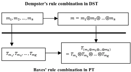
, , … , …
, , … , … …
Dempster’s rule combination in DST
Bayes’ rule combination in PT
Table 4 Survey of the mappings and their properties.
P. 5
P. 4
P. 3
P. 2
P. 1
NO NO NO NO NO
.
NO NO NO NO NO
NO YES YES YES YES
NO NO NO NO NO
NO NO NO NO NO
NO NO NO NO NO
NO NO NO NO NO
NO NO NO NO NO
NO NO NO NO NO
The results are summarized in Table 4. As a consequence two important results are extracted from the Table 4.
1. The independency from the Dempster’s rule of combination of a probability transformation will also involve the last three conditions. So two main requirements for a conversion from the DST to the PT are invariance with respect to the marginalization and invariance with respect to the Dempster’s rule of combination.
2. According to the Table 4, it can be seen that only the normalized plausibility transformation satisfies four of the five conditions. In other words, if we want to choose the most justifiable mapping through the mentioned transformations, the normalized plausibility transformation is the best choice. Also the invariance with respect to marginalization problem of this mapping will be remained. This issue will be proven in the next sections.
4 Solving the Problem of the Invariance with Respect to the Marginalization Process
Invariance with respect to the marginalization process means that the marginal probability distribution of the joint probability transformation is equal to the probability distribution of the marginal BPAs. In this subsection, we will examine the reasons for the dependency of the pignistic probability and the normalized plausibility transformation on the marginalization process. To this end, we need to focus on the projection method in DST. The classic projection process in DST loses some probabilistic information, as shown in Example 7.
Example 7. If , , , : 2Ω 0,1 are four different joint BPAs with , and
, , .
Z , Z , Z , Z , Z , Z
Z 1 ,
Z , Z , Z , Z
Z 1 (20) Z , Z
Z 1 ,
Z , Z , Z , Z
Z 1
Then, there are different BPAs with different focal elements and we have,
Z , Z , Z , Z , Z , Z
Z , Z , Z , Z Z , Z (21)
Z , Z , Z , Z ,
Therefore, the projections of different subsets with different numbers of marginal singletons (three and three for the first subset, two and two for the second subset, one and one for the third subset, and three and one for the fourth subset) are equal. The four marginal BPAs on are thus equal and can be given by:
,
1 (22)
, ,
, ,
(23)
In this example, there are four joint BPAs with different s, although their marginal pignistic probabilities computed from the marginal BPAs are equal. Additionally, there are four joint BPAs with different s, although their marginal normalized plausibility transformations computed from the marginal BPAs are equal.
In other words, in the standard projection process, the number of marginal singletons ( and ) that exists in the joint state space is not taken into account. This point explains why and are not invariant under the marginalization process. To solve this problem, we need to consider the number of marginal singletons in the projection process. Therefore, we try to retain this information by defining the Projection Set and rewriting the marginalization formula as follows:
Definition 20. If : 2 XY 0,1 is the joint BPA
on XY, then the Projection Set of XY on , is shown by , which is the set of all joint state space members such that and is given by:
| , (24) Definition 21. If : 2 0,1 is the joint BPA defined on ΩXY, then the marginal of over based on is denoted by ḿXYΩX, and is computed as
follows:
́ (25)
It should be noted that the results of the new marginalization procedure are almost identical with the classical method of the marginalization in Dempster-Shafer theory, only the formula has been little changed. Based on these changes, the pignistic probability and the normalized plausibility transformation could be modified as follows:
Definition 22. If : 2 XY 0,1 is a joint BPA
defined over , then the modified pignistic probability is defined for each singleton Ω and
Ω as follows:
. | |
,
(26)
, | |
,
, (27) where is the number of in the subset and | | denotes the cardinality of .
Definition 23. If : 2 XY 0,1 is a joint BPA
on ., then the modified normalized plausibility transformation is defined for each singleton Ω
and Ω as follows:
1
∆ , .
(28)
, 1
∆
,
, (29) where, Δ is the normalization factor.
Corollary 1 In one-dimensional state space,
1- The modified pignistic probability is reduced to the pignistic probability, i.e.,
.
2- The normalized plausibility transformation and the modified normalized plausibility transformation are equal ( ).
Proof: In one-dimensional space we have,
:
1 and (30) Then,
. | |
,
| |
,
(31)
and,
1
∆ , .
1
∆ ,
(32)
Here, the invariance with respect to marginalization of the modified pignistic probability is expressed in the following proposition and its proof is given in Appendix A.
Proposition 1. Let : 2 0,1 be a joint BPA over ΩXY, be the joint modified pignistic probability and be the modified pignistic probability of marginal , then we have:
(33) Proof: See Appendix A.
Now, invariance with respect to marginalization of is expressed with the following proposition: Proposition 2. Let : 2 0,1 be a joint BPA on ΩXY, be the joint modified normalized plausibility transformation and be the modified normalized plausibility transformation of marginal , then we have:
(34) Proof: See Appendix B.
To clarify the point, the modified pignistic probability and the modified normalized plausibility transformation are computed for the BPAs of Example 2.
First, the joint probabilities are computed as follows:
/3 /3
/3 1 (35)
, , 1 2 1 2
1 2
1
1 2
(36)
As it can be seen in the Table 5, both the modified pignistic probability and the modified normalized plausibility transformation are invariant under the
marginalization process ( ,
, and
).
Example 8. If : 2Ω 0,1 is a joint BPA on
, , and , , then we need to
check the invariance with respect to marginalization
concept for , , and .
The joint state space is:
Z , Z , Z , Z , Z , Z .
, , , ,
,
, , ,
, , 1 ,0 1
(37)
Table 5 Projection Sets of X and Y, corresponding modified pignistic probabilities and modified normalized plausibility transformation.
.
2Ω
X
.
2Ω
2a 1 2a 2a/3
2a 1 2a 2a/3
1 1 2a
1 2a/3
1 1 2a
1 2a/3
… ...
, ,
… …
, ,
First, we compute the joint probabilities as follows:
, ,
27 240
27 240
80 53
240
60 240
80 23
240
80 38
240
(38)
, ,
2 12
2 12
4 2
12 12
4 12
4 2
12
(39)
Then, marginal BPAs of X, , ,
, and are calculated (Table 6). In the next
step, the marginal BPA of Y, , , ,
and are computed (Table 7). Finally, a comparison will be made between the results of Table 6 and Table 7, suggesting that:
, (40)
, (41)
But,
, (42)
, (43)
and,
, (44)
,
(45) but,
, (46)
, (47)
Table 6 Marginal X,the Projection Set of X, , , , and .
.
. 2
4 12 54
240 2
8 2
12 0
4
12
80 7
240
4 a
8
6 a
12 4
8 3
12
160 61
240 ,
4 a
8
6 a
12 4
----
----
--- 0
----
----
--- 0
----
----
, ,
--- 1
----
----
, , , ,
, , ,
--- 2
4
Table 7 Marginal Y, the Projection Set of Y, , , , and .
. Y .
2Ω
8
12
160 49
240 4
8
4 8 0
4
12
80 49
240 4
8
4 8 4
---- ----
, , , , , ,
, , , , , ,
---- ----
1 4
5 Applications of the Proposed Mappings
Computing the amount of uncertainty or information contained in an event is of crucial importance in many applications in decision-making systems. To calculate the amount of uncertainty, we need to define a measure. Shannon entropy (H(x)) is an uncertainty measure in PT proposed by Shannon [24]. The different types of uncertainty proposed in various theories have been classified by Klir and Yuan in [25]. Dempster-Shafer Theory is an extension of the probability theory and the set theory, and as such, it is able to represent two types of uncertainty, i.e., nonspesifity and discord. Klir proposed AU as an aggregated uncertainty measure that computes nonspecificity and discord simultaneously [9]. He posited that any aggregate uncertainty measure such as AU must satisfy five requirements including Probability consistency, Set consistency, Range, Subadditivity and Additivity. Jousselme et al. proposed another aggregated uncertainty measure called AM based on the pignistic probability [13]. They proved that AM satisfies the five requirements of an aggregate uncertainty measure. But, Klir and Lewis showed that the proof of AM subadditivity provided by Jousselme et al. was wrong [14]. They referred to the dependency of the pignistic probability on the marginalization process to support their argument.
Similar to the pignistic probability that is used in AM, we can exploit the other DST to PT transformations to measure the amounts of ambiguity in DST. But the Table 3 indicates that the all mapping are dependent to the marginalization process and so the corresponding ambiguity measures are not subadditive. In Section 4, we proposed and that are invariant under the marginalization process and so are adequate to use in the ambiguity measure. Therefore the ambiguity measures based on and will be subadditive.
Now, similar to the entropy measure in PT, we have two new aggregate uncertainty measures in DST for computing the amounts of ambiguity. The question is where can be used these ambiguity measures. We attempted to use these measures for computing the amounts of dependency between two variables. As we know, mutual information (MI) as a tool for measuring the dependency between two variables is used in many applications in probability theory [26]. Similar to the mutual information in probability theory, the mutual ambiguity based on and can be used for computing the dependency between two variables in DST.
Shahpari et al. in [27], used the mutual ambiguity measure based on called , in a threat assessment problem constructed by a Dempster-Shafer network. In their paper, MAM is used for computing the influence of the network input variables to the threat value.
In the similar way, we introduce the ambiguity measure and the mutual ambiguity measure based on
and as follows:
Definition 24. If : 2Ω 0,1 is a BPA on and and are DST to PT transformations, then the corresponding ambiguity measures are given by:
. log
(48)
. log
(49)
Definition 25. If : 2 XY 0,1 is an arbitrary
joint BPA on XY, the associated marginal BPAs are X and Y, then mutual ambiguity measures based on
and , are given by:
;
, (50)
;
, (51)
Example 9. Let us consider the issue of the social bliss and the factors that affect a person’s happiness. Suppose that there are five independent parameters such as social acceptability (SA), hope for the future (HF), poverty (P), feeling of security (FS), and fulfillment of emotional needs (FE). The relationships between these factors and the target variable, social bliss (SB), are modeled by the expert knowledge expressed by some rules. Then according to the implication rule in [28-29], each of the rules can be represented by a BPA.
For example, an expert explains his opinion about the effect of social acceptability on the social bliss in the following two rules: 1) if the person has a good level of acceptability, then with certainty between 0.5 to 0.8 he feel happiness; and 2) if the person has no social acceptability, then with certainty between 0.3 to 0.6 he does not feel happiness. To model these rules, suppose
that the state space of SA is 0, 1
and the state space of SB is 0, 1 . Now, These rules are rewritten as: “(SA=1)Æ(SB=1) with confidence between 0.5 to 0.8.” and “(SA=0)Æ(SB=0) with confidence between 0.3 to 0.6.” Then, according to the implication rule in [28] the joint BPA is computed as follows:
The joint state space will be the power set of
, 0,0 , 0,1 , 1,0 , 1,1
, , , and we have,
, , 0.06
, , 0.08
, , , 0.06
, , 0.15
(52)
, , 0.2
, , , 0.15
, , , 0.09
, , , 0.12
, , , , 0.09
Similar to the above modeling, the state space of HF is 0, 1 and the expert rules and the joint BPAs are given as follows:
(SA=1)Æ(SB=1) with confidence between 0.5 to 0.8.
(SA=0)Æ(SB=0) with confidence between 0.3 to 0.6.
, , 0.05
, , 0.02
, , , 0.03
, , 0.4
, , 0.16
, , , 0.24
, , , 0.05
, , , 0.02
, , , , 0.03
(53)
For FE with the state space 0, 1
we have,
(FE=1)Æ(SB=1) with confidence between 0.6 to 0.7.
(FE=0)Æ(SB=0) with confidence between 0.2 to 0.5.
, , 0.02
, , 0.03
, , , 0.05
, , 0.12
, , 0.18
, , , 0.3
, , , 0.06
, , , 0.09
, , , , 0.15
(54)
For FS with the state space 0, 1 , the expert knowledge and the joint BPA are given by:
(FS=1)Æ(SB=1) with confidence between 0.2 to 0.5.
(FS=0)Æ(SB=0) with confidence between 0.9 to 0.98.
, , 0.27
, , 0.024
, , , 0.006
, , 0.18
, , 0.016
, , , 0.004
, , , 0.45
, , , 0.04
, , , , 0.01
(55)
Finally, for P with the state space
0, 1 we have,
(P=0)Æ(SB=1) with confidence between 0.6 to 0.8. (P=1)Æ(SB=0) with confidence between 0.7 to 0.9.
, , 0.12
, , 0.42
, , , 0.06
, , 0.04
, , 0.14
, , , 0.02
, , , 0.04
, , , 0.14
, , , , 0.02
(56)
Now, we want to identify which variables of the problem are more influential on the social bliss. To this
end, ; and ; are employed to
compute the dependency of the paired variables (SA,SB), (HF,SB), (FE,SB), (FS,SB), and (P,SB). From Table 8 it can be observed that HF has most influence to the bliss and SA has minimum effect.
6 Conclusion
In this paper, the necessary conditions that were suggested by Cobb and Shenoy are studied for nine different mappings from DST to PT. The results indicate that only the normalized plausibility transformation can meet four conditions among five and the rest of mappings satisfy none of the conditions. Another important point is that the condition of invariance with respect to the marginalization process does not exist for any mappings. In this study, we took a closer look at the projection method in DST, finding
Table 8 mutual ambiguity of the paired variables of Example 9.
(SA,SB) (HF,SB) (FE,SB) (FS,SB) (P,SB)
; 0.0060 0.1757 0.0255 0.1218 0.1371
; 0.0044 0.1457 0.0192 0.1210 0.1152
that some probabilistic information is lost in the marginalization process. This problem solved by introducing a Projection Set to retain the probabilistic information. Then, and which are invariant under the marginalization process was proposed. Similar to the AM that uses the pignistic probability, these modified mappings were utilized in two new ambiguity measures called MAM and
. MAM and against AM are
subadditive because and are independent from the marginalization process. Based on MAM and , the concept of mutual ambiguity were defined in DST. As an application, the mutual ambiguity
measures, ; and X; Y are
employed in a social bliss problem to compute the dependency of the variables to the person’s happiness. According to many applications of the mutual information in PT, these mutual measures can be used in the future by researchers in various applications.
Appendix A
Proof of proposition 1:
We must prove that ∑| | ,
.We start from the left of term,
, | |
| | ,
| |
| |
, ,
| |
| |
, , | |
| |
, ,
| |
| |
, , | |
| |
| | ,
(A1)
2 | |
,
| |
| | | | ,
. | | ,
In line 3, for the first term we have,
| |
, ,
| |
| |
, ,
| | , |Y| ,
| | ,
(A2)
For the second term we have,
| |
, ,
| |
| |
, ,
| | , |Y| ,
2
| | ,
(A3)
This equation is explained with following example:
If X , and Y , are the state
spaces of and , the joint state space in DST is 2 XY
and has 2 16 members. For simplicity we use another notation as follows:
Z , Z , Z , Z . We have two term in the right side of above equation as follows (because, | | 2):
| |
, ,
| |
, ,
(A4)
Then, we must compute the summation of in two subsets and such that:
| , , , 2
Z , Z , Z , Z , Z , Z , Z , Z ,
Z , Z , Z , Z (A5)
and,
| , , , 2
Z , Z , Z , Z , Z , Z , Z , Z ,
Z , Z , Z , Z (A6)
It is clear that,
|
2 , (A7)
So, this two terms is equal to,
2
| |
, (A8)
Similar to before for the third term we have,
| |
, , | |
| |
| |
, , | |
| |
, |Y| , | |
| |
| | | | ,
(A9)
So, the modified pignistic probability is invariant under the marginalization process.
Appendix B
Proof of proposition 2:
We must prove that ∑| | ,
.We start from left of term,
, | |
1 ∆
, | |
1 ∆
, ,
| |
, , | |
1 ∆
, ,
| |
, , | |
| |
1 ∆
, 21
∆ ,
| |1 ∆
| | ,
1
∆ .
,
(B1)
In line 3, for the first term we have,
, ,
| |
, ,
, |Y| ,
,
(B2)
For the second term we have
, ,
| |
, ,
, |Y| , 2
,
(B3)
This equation is explained with the similar example given in the appendix A.
If X , and Y , are the state
spaces of and , the joint state space in DST is 2 XY
and has 2 16 members. For simplicity we use another notation as follows:
Z , Z , Z , Z . We have two term in right side of above equation as follows (because, | | 2):
, ,
, ,
(B4)
Then, we must compute the summation of in two subsets and such that:
| , , , 2
Z , Z , Z , Z , Z , Z , Z , Z ,
Z , Z , Z , Z (B5)
And,
| , , , 2
Z , Z , Z , Z , Z , Z , Z , Z ,
Z , Z , Z , Z (B6)
It is clear that,
|
2 , (B7)
So, this two terms is equal to,
2
, (B8)
Similar to before we have,
, , | |
| |
, , | |
, |Y| , | |
| |
| | ,
(B9)
So, the modified normalized plausibility transformation is invariant under the marginalization process.
References
[1] J. Sudano, “Yet Another Paradigm Illustrating Evidence Fusion”, In Proceedings of Fusion 2006 International Conference on Information Fusion, Firenze, Italy, 2006.
[2] F. Cuzzolin, “Two new Bayesian approximations of belief functions based on convex geometry”, IEEE Trans. on Systems, Man, and Cybernetics part B, Vol. 37, No. 4, pp. 993-1008, 2007. [3] P. Smets, “Constructing the pignistic probability
function in a context of uncertainty”, M. Henrion, R. D. Shachter, L. N. Kanal, J. F. Lemmer (Eds.), Uncertainty in Artificial Intelligence, Vol. 5, pp. 29–40, 1990.
[4] P. Smets, “Decision making in a context where uncertainty is represented by belief functions”, R. P. Srivastava, T. J. Mock (Eds.), Belief Functions in Business Decisions, pp. 316–332, 2002.
[5] P. Smets, “Decision making in the TBM: the necessity of the pignistic transformation”, International Journal of Approximate Reasoning, Vol. 38, No. 2, pp. 133–147, 2005. [6] P. Smets and R. Kennes, “The transferable belief
model”, Artificial Intelligence, Vol. 66, No. 2, pp. 191–234, 1994.
[7] F. Smarandache and J. Dezert, Applications and Advances of DSmT for Information Fusion, American Research Press, Rehoboth, Vol. 3, 2009.
[8] G. J. Klir, Uncertainty and Information: Foundations of Generalized Information Theory, Hoboken, NJ: Wiley Inter science. J., 2006. [9] G. J. Klir and M. J. Wierman, Uncertainty-Based
Information, Studies in Fuzziness and Soft Computing, Vol. 15, 1999.
[10] Y. Maeda, H. T. Nguyen and H. Ichihashi, “Maximum entropy algorithms for uncertainty measures”, International Journal of Uncertainty,
Fuzziness & Knowledge-Based Systems, Vol. 1, No. 1, pp. 69-93, 1993.
[11] D. Harmanec and G. J. Klir, “Measuring total uncertainty in Dempster-Shafer theory”, International Journal of General Systems, Vol. 22, No. 4, pp. 405-419, 1994.
[12] J. Abellán and S. Moral, “Completing a total uncertainty measure in the Dempster–Shafer theory”, International Journal of General Systems, Vol. 28, No. 4–5, pp. 299–314, 1999. [13] A. L. Jousselme, C. Liu, D. Grenier and É.
Bossé, “Measuring ambiguity in the evidence theory”, IEEE Transactions on Systems, Man and Cybernetics part A: Systems and Humans, Vol. 36, No. 5, pp. 890–903, 2006.
[14] G. J. Klir and H. W. Lewis, “Remarks on measuring ambiguity in the evidence theory”, IEEE Transactions on Systems, Man and Cybernetics part A: Systems and Humans, Vol. 38, No. 4, pp. 995-999, 2008.
[15] B. R. Cobb and P. P. Shenoy, “A comparison of Bayesian and belief function reasoning”, Information Systems Frontiers, Vol. 5, No. 4, pp. 345–358, 2003.
[16] B. R. Cobb and P. P. Shenoy, “On transforming belief function models to probability models”, Working Paper, school of Business, University of Kansas, Lawrence, KS, No. 293, 2003.
[17] B. R. Cobb and P. P. Shenoy, “A comparison of methods for transforming belief function models to probability models”, In T. D. Nielsen, N. L. Zhang, eds., Symbolic and Quantitative Approaches to Reasoning with Uncertainty, Lecture Notes in Artificial Intelligence, Vol. 2711, pp. 255–266, 2003.
[18] B. R. Cobb and P. P. Shenoy, “On The Plausibility Transformation Method for Translating Belief function Models to Probability Models”, Int. J. of Approximation Reasoning, Vol. 41, No. 3, pp. 314-330, 2006. [19] A. Dempster, “Upper and lower probabilities
induced by multivalued mapping”, Annals of Mathematical Statistics, Vol. 38, No. 2, pp. 325– 339, 1967.
[20] G. Shafer, A Mathematical Theory of Evidence, Princeton University Press, Princeton, 1976. [21] A. Dempster, “New methods of reasoning
toward posterior distributions based on sample data”, Annals of Mathematical Statistics, Vol. 37, No. 1966, pp. 355-374, 1987.
[22] J. Sudano, “Pignistic Probability Transforms for Mixes of Low and High Probability Events”, In Proceedings of Fusion 2001 Int. Conf. on Information Fusion, Canada, August 2001. [23] F. Voorbraak, “A computationally efficient
approximation of Dempster-Shafer theory”, International Journal of Man-Machine Studies, Vol. 30, No. 5, pp. 525–536, 1989.
[24] C. E. Shannon, “A mathematical theory of communication”, The Bell System Technical Journal, Vol. 27, No. 3, pp. 379-423, 1948. [25] G. J. Klir and B. Yuan, Fuzzy Sets and Fuzzy
Logic: Theory and Applications, Upper Saddle River, NJ: Prentice-Hall, 1995.
[26] T. M. Cover and J. A. Thomas, Elements of Information Theory, John Wiley, New York. 1990.
[27] A. Shahpari and S. A. Seyedin, “Using Mutual Aggregate Uncertainty Measures in a Threat Assessment Problem Constructed
by
Dempster-Shafer Network”, IEEE Transactions on Systems, Man and Cybernetics, Vol. 44, No. 12, pp. 1, 2014.[28] A. Benavoli, B. Ristic, A. Farina and L. Chisci, “An application of evidential networks to threat assessment”, IEEE Trans. Aerospace and Electronic Systems, Vol. 45, No. 2, 2009.
[29] B. Ristic and P. Smets, “Target identification using belief functions and implication rules”, IEEE Trans. Aerospace and Electronic Systems, Vol. 41, No. 3, pp. 1097–1103, 2005.
Asghar Shahpari received his B.Sc.
degree in Electrical Engineering from Shahroud University of Technology in 1999 and M.Sc. degree in Communication Engineering from Ferdowsi University of Mashhad in 2001 respectively. Currently, he is pursuing the Ph.D. degree in Communication Engineering at Ferdowsi University of Mashhad. His research interests are in the field of data fusion, Evidence theory, uncertainty, advanced signal processing techniques and pattern recognition area.
Seyed Alireza Seyedin received the
B.Sc. degree in Electronics Engineering from Isfahan University of Technology, Isfahan, Iran in 1986, the M.Sc. degree in Control and Guidance Engineering from Roorkee University, Roorkee, India in 1992, and the Ph.D. degree from the University of New South Wales, Sydney, Australia in1996. Since 1996, he has been with the faculty of engineering, Ferdowsi University of Mashhad, Mashhad, Iran as an assistant professor and since 2007 as an associate professor. He was the head of the department of the electrical engineering for the period 1998-2000. He is a member of technical committee of the Iranian Conference on Machine Vision and Image Processing (MVIP). Dr. Seyedin's research activities focus on the Machine vision, DSP-based signal processing algorithms and digital image processing techniques.