International Journal of Finance and Managerial Accounting, Vol.3, No.12, Winter 2019
1
With Cooperation of Islamic Azad University – UAE BranchNonlinear Model Improves Stock Return Out of Sample
Forecasting (Case Study: United State Stock Market)
Zahra Farshadfar
Department of Economics, College of Humanities, Kermanshah Branch, Islamic Azad University, Kermanshah, Iran (Corresponding Author)
Marcel Prokopczuk
Institute for Financial Markets, Leibniz University Hannover, Hannover, Germany.
ABSTRACT
Improving out-of-sample forecasting is one of the main issues in financial research. Previous studies have achieved this objective by increasing the number of input variables or changing the kind of input variables. Changing the forecasting model is another possible approach to improve out-of-sample forecasting. Most researches have focused on linear models, while few have studied nonlinear models. In the present study, we have reduced the number of variables and at the same time applied a nonlinear forecasting model. Oil prices have been used as predictors to predict return by application of a new artificial neural network nonlinear model named Deep Learning and its comparison with OLS and ANN methods. Results indicate that the applied non-linear model has higher accuracy compared to historical average model, OLS and ANN. It also indicates that out-of-sample prediction improvement does not always depend on high input variables numbers. On the other hand when using a smaller number of input variables, it is possible to improve this forecasting capability by changing the model and applying nonlinear models.
Keywords:
1. Introduction
Predictability of stock market has been under academic and professional attention for many years (Campbell, 2012). Historical research has been done for many reason; first of all, it decreases risks by increasing return prediction ability. Therefore, research in the scope of financial market predictability is very important for private investors and institutional investors. Portfolio return predictability is also important for corporate presidium whose intention and motion specify perceived value of companies. Market predictability may also be used to model the development of the stock market which is important for stock market operators and supervisors. Finally, while opinions on the efficiency of markets vary, many widely accepted empirical studies show that financial markets are to some extent predictable (Bollerslev et al., 2014; Phan et al., 2015) and market predictability doesn’t confirm the Efficient Market Hypothesis which is an embossing assumption in many financial model. These forecasting may have been conducted to forecast the main important variables such as price, return and volatility. The main point is when the goal is to improve return prediction (especially on out of sample data), most researches are trying to overcome this problem by changing either the variables or increasing them. The most variable increment to out of sample prediction is observed in Goyal kitchen regression1. Less research has focused
on model changing to improve out of sample prediction or if this has happened, most of the applied models have been linear and few have considered nonlinear models. Despite the fact that research show many factors affect stock market’s performance, fluctuations in the stock market are non-linear (Jasemi
et al., 2011). In cases where non-linear models are used, less attention is paid to economic theories. In fact, there is a gap between application of nonlinear models and economic theories. Some research have imposed economic constraints on return time series data, particularly when the data are noisy and parameter uncertainty is a concern as in return prediction models. Economic constraints have formerly been found to improve asset return forecasts, while no broad consensus exists on how to impose such constraints (Pettenuzzo et al., 2014)
In this study, we want to see if out-of-sample prediction improvement does not only depend on increase in the number of input variables and besides
that, can sometimes better result be obtained by choosing less but correct number of variables as well as changing the model. In the present paper, further insights for the crude oil and stock market relationship are employing by an out-of-sample analysis utilizing a recently developed of artificial neural network called ‘Deep Learning Algorithm’ to show how well the oil price forecasts stock returns. Then the robustness of forecasting performance has been evaluated by allocation of different forecasting model at different data frequencies to see if the results depend only on the data frequency or also on the model.
2. Literature review
A review of literature on return shows that return forecasting study can be categorized as three aspects:
First: Model type and estimation method: It has been suggested for a long time that return can be predicted using different kind of methods mainly classified as time series forecasting models. These model can be divided in two big categories: classical models or econometrical models, that more than of them are liner, and modern model that most of them are nonlinear and usually originate from other disciplines such as mathematics, physics, computer and etc. (For example: Adebiyi et al., 2014; Kim and Enke, 2016a; 2016b; Rather et al., 2017). Empirical studies result on return forecasting models are different. Some of them propose nonlinear models do not perform linear models (for example: Lee et al., 2007; Lee et al., 2008), some others show linear models outperform or perform as well as nonlinear models (for example: Agrawal et al., 2013; Adebiyi et al., 2014), and finally some studies find nonlinear models outperform linear models (for example: Enke and Mehdiyev, 2013; Rather et al., 2017).
In this research we choose non liner model. Although stock market is a non-linear dynamic system and predicting the stock prices path is a difficult task, but there is uniform agreement that stock returns behave nonlinearly (Chong et al., 2017, Ahmadi et al., 2018) and if we show this nonlinear behavior linearly, the model has not been chosen correctly and we encounter model specification Error problem.
but it owes its popularity to its ability to fit into any functional data relationship to an arbitrary degree of exactness and works best in circumstances where financial theories have virtually nothing to say about likely functional form for the relationship between a set of variables (Brooks, 2015). In addition, this model can discover the complex nonlinear relations and handle the predominant uncertainty and inaccuracy in the stock market (Ahmadi et al., 2018(. Despite its abilities, this model has not been very privileged among economists. Studies have shown that this model has not succeeded in predicting out-of-sample data. Therefore, in order to obtain a better result, this model is usually combined with other nonlinear models like fuzzy family model or genetic algorithm, etc. This combination improves the model's performance and at the same time, it increases the complexity of the method too. In the present study, we have chosen ‘Deep Learning Algorithm’ from the many available kind of intelligence algorithm. There are some reason for this choice: initially, deep learning is one of the machine learning algorithms which has received considerable attention in recent years. There seems to be increasing interest in whether deep learning can be efficiently applied to financial problems. But the literature (at least in the public domain) still remains limited. Second: classical ANN models have structural problems such as gradient vanishing that doesn’t allowed the researcher to increase the layer or node and random weighting to the first layer parameter and vice versa. These problems have limited the forecasting ability of the model. The mentioned have been solved in deep learning method. In fact, this method offers an innovative technique that does not necessitate a pre-specification during the modeling process as they independently learn the relationship characteristic in the variables (Chong et al., 2017). Finally, every day many data are generated in financial markets, that affects investors' expectations, supply, demand, and ultimately prices. In classical models it is impossible or very difficult to study these data simultaneously and when it has been done, it is difficult to provide model presumptions as many of the data’s information disappears. Deep learning is nonlinear data based method that takes huge amount of data as input and then extracts information from them. This is why this model is usually used in condition that using true preprocessing data methods can keep many of data related information.
Second: Kind and number of variables:
Forecasting in the financial time series is basically predicting the series behavior one or few steps ahead with the help of a number of variables. The variables used for forecasting are either economic2 or financial variables3 or in some cases, technical analysis output (Brock et al., 1992). In some studies, these variables are used in combination (Welch and Goyal, 2008; Rapach et al., 2010). One of the benefit of variable combination is obtaining information from many economic and financial variables and at the same time forecast volatility reduction (Phan et al., 2015). It has to be mentioned that even though financial and economic data are different in nature, their combination should be done with caution.
price (which negatively affects economic growth) will in turn have a negative effect on the stock market (Narayan and Sharma, 2011). While this relationship was particularly accepted for the United States of America, a recent study by Narayan et al. (2014) showed the relevance of oil prices for 45 developed and developing countries. There are many reasons for the impact of oil price on macroeconomic variables and consequently economic growth. The first reason is that oil is the main input in production process and when oil prices rise, the cost of production increases. Therefore, it is not surprising when Hamilton (1983) points out that seven of the eight post-war recessions in the United States has preceded sharp rises in oil prices. This implies that oil is almost always at the purview of policymakers. The second reason is related to the treatment of crude oil as an asset class. Some studies (like Narayan et al., 2014) show how investing in oil can be profitable and demonstrate that oil investment is therefore at the heart of commodity-based investment. This demonstrates that oil is also in the purview of investors. Finally, it has to be mentioned that focus and emphasis on oil prices is unrelenting and the above stated characteristics of crude oil demonstrate its economic importance in financial markets and market return.
Third: Type of prediction or the ability to predict in-sample and out-of-sample data:
Literature demonstrate relatively limited evidence of predictability using out-of-sample tests. The results show that the evidence for stock return predictability (in US market) is for most parts in-sample; and it is not robust to out-of-sample evaluations (Goyal and Welch, 2003; Brennan and Xia, 2005; Butler et al., 2005; Ang and Bekaert, 2007). Some researchers such as Tashman (2000) claim that forecasting methods should be considered for accuracy using out-of-sample tests rather than goodness-of-fit to past data (in-sample tests). Additionally, Welch and Goyal (2008) mentioned that a predictor must deliver a good out-of-sample predictive performance in order to be used by an investor. The out-of-sample forecasting analysis would be more relevant for investors as they are required to take decisions in real time. In the present study, have we focused on out of sample prediction. In addition to the above reasons, the main feature of recent study on oil prices is that they typically focus on in-sample predictability while nothing is understood
about how well the oil price predicts out-of-sample stock returns.
Another thing that would be consider is data frequencies. Actually there is no theory that express frequency choice4. Different literature have been used for data frequencies in the stock returns forecasting. This is understandable because predicting is assumed for a purpose which dictates the choice of data frequency. Weekly, monthly and annual data have been used for stock return predictability. Therefore, it seems that one should confirm the robustness of the forecasting performance by using data at different frequencies (Phan et.al, 2015). This is not a unimportant issue because previous studies demonstrate that the choice of data frequency does matter5.
Most research constructed on out-of-sample forecasting of stock returns use low-frequency data such as annual data (Welch and Goyal, 2008), quarterly data (Rapach et al., 2010), or monthly data (Kong et al., 2011; Westerlund and Narayan, 2012). This paper investigates stock return predictability using a crude oil price as predictor that has higher frequency data available. This allows to capture some better insights due to the ability to forecast at short-horizon for stock return predictability. In this research we have use daily, weekly and monthly data frequencies.
3. Methodology
3.1. The framework
Previous study such as Rapach et al. (2010) and Westerlund and Narayan (2012) have tested the stock return predictability based on the simple predictive regression model as follow:
(1)
where 𝑟𝑡+ℎ is the excess stock return, measured as
stock returns in excess of the risk-free rate and xt is the
predictor variable (in this study oil price).
The predictive ability of 𝑥𝑡 can be tested under the null and alternative hypothesis as follow:
{ (2)
Although this model is simple to estimate, Phan et al.
persistency, and heteroscedasticity issues. This while, the mentioned problem have been solved for machine learning models6.
In this research we have use this predictive regression as follow: first, we have use it for estimating traditional linear model, OLS to compare it with nonlinear models. Second, search a predictor function f in order to predict the market return at time t+1 , rt+1 ,
given the features (representation ) ut extracted from
the information available at time t. We assume that rt+1
can be disjointed into two parts: the predicted output
̂t+1 = f (ut), and the unpredictable part γ, which we
regard as Gaussian noise:
rt+1 = ̂t+1 + γ, γ∼N (0 , β) (3)
Where N (0, β) denotes a normal distribution with zero mean and variance β. The representation ut can be
either a linear or a non- linear transformation of the raw level information Rt. Denoting the transformation
function by φ, we have:
ut = φ(Rt ) (4)
̂t+1= f◦φ(Rt ) (5)
3.2. Deep learning
Artificial Neural Networks is a subset of machine learning and machine learning is the subset of artificial intelligence. In the old literature define ANNs as a class of models whose structure is largely inspired by the way that brain performs computation. But recent literature don’t compare ANN’s with brain. They call it the computational methods who had worked with many layers.
There many kinds of ANNs exist. They can be categories in several ways, but the main structure of them is the same. All kinds of ANN consist of one or more layer and each layer consist of one or more Neuron. Each Neuron have 4 parts: input, weight matrix, activation function and output. Network can be trained by three methods. If input data are labeled, output data are specified for input matrix, all models and methods are define by the user then the network just implements the program and this kind of train is called supervised learning. If input matrix is not labeled and allows the network to take feature from the data, this kind of training is called unsupervised
learning. In financial studies supervising learning is usually used. The nonlinear relationship between two variables hl and hl+1 is specified by neural network
through a network function, which typically has the form of:
h l+1 = δ(W hl + b) (6)
In which, δ is called an activationfunction, and the matrix W and vector b are model parameters. The variables hl and hl+1 are said to form a layer; when
there is only one layer between the variables, their relationship is called a single-layer neural network.
Multi-layer neural networks augmented with advanced learning methods are generally referred to as deep neural networks (DNN). DNN for the predictor function, y = f(u), can be constructed by serially stacking the network functions as follows:
h1 = δ1 (W1u+ b1)
h2 = δ2 (W2 h1 + b2)
…...
y = δL (WL hL−1 + bL) (7)
Where L is the number of layers.
Given a dataset {un ,τn }Nn =1 of inputs and targets, and
an error function ԑ(yn , τn) that measures the difference between the output yn = f(un ) and the target τn , the model parameters for the entire network, θ= {W1,…,
WL , b1,…,bL}, can be chosen so as to minimize the
sum of the errors:
[ ∑ ( )
] (8)
Given an appropriate choice of ԑ (·), its gradient can be obtained analytically through error back propagation (Bishop, 2006). In this case, the minimization problem in (8) can be solved by the usual gradient descent method. A typical choice for the objective function that we adopt in this paper has the form:
∑ ‖ ‖ ∑ ‖ ‖ (9)
Where ‖ ‖ and ‖ ‖ respectively denote the Euclidean norm and the matrix L2 norm. The second term is a
3.3 Training deep neural networks
We constructed the predictor functions, ̂ ( ) . Using DNN, we employ a three-layer network with 100 nodes in hidden three-layers of the form:
h1 = ReLU(W1 ut + b1)
h2 = ReLU(W2 h1 + b2)
̂i,t+1 = W3 h2 + b3 (10)
Where ReLU is the rectified linear unit activation function defined as: ReLU(x) = max (x, 0) with max being an element-wise operator. ReLU is known to provide a much faster learning speed than standard sigmoid units, while maintaining or even improving the performance when applied to deep neural networks (Nair and Hinton, 2010). Nevertheless, we also test a standard ANN for comparison: we replace ReLU with a sigmoid unit and reduce the nodes in hidden layers to one and keep the rest of the settings and parameters equal. With one sets of features, Raw Data, as the input, the DNN is trained minimizing the objective function defined in Eq. (9) with 1000 learning iterations (epochs), and the regularizer coefficient, λ=0.001. The last 20% of the training set is used as a validation set for early stop- ping to avoid over fitting. The training was conducted using keras in Anaconda 3, Python 3.6.
3.4. Benchmark model
Following previous studies such as Welch and Goyal (2008) and Rapach et al. (2010), we use historical average model as bench mark model:
̂ ∑ (11)
3.5. Statistical evaluation
Between various models, MSFE is the most popular metrics in order to evaluate the forecast accuracy. This model (MSFE) which is computed as below has been widely used in the stock return forecasting literature.
∑ ( ̂ ) (12)
where 𝑇0 and P are the number of in-sample and out-of-sample observations, ̂ is the estimated
stock return from the predictive regression model and
is the actual stock return. Campbell and
Thompson (2008) introduced out-of-sample R2 statistic is a simple statistic for comparing the MSFE of the benchmark model (𝑀𝑆𝐹𝐸0) and the MSFE of the competitor model (𝑀𝑆𝐹𝐸1), it is computed as:
(13)
The measures the reduction in MSFE for the
competitor model compared to the benchmark model. If the competitor model’s MSFE is less than that of the benchmark model ( > 0), it indicates that the
competitor model is more accurate in forecasting than the benchmark model, and vice versa. There are other relatively traditional tests that allow us to evaluate the statistical significance of the MSFE from any other models. For example, one can test the null hypothesis
𝐻0∶ 𝑀𝑆𝐹𝐸0 ≤𝑀𝑆𝐹𝐸1 against 𝑀𝑆𝐹𝐸0>𝑀𝑆𝐹𝐸1, corresponding to 𝐻0∶ 𝑅𝑂𝑆2 ≤0 against 𝑅𝑂𝑆2>0. The most popular method in this regard is Diebold and Mariano’s (1995) and West (1996) statistic (DMW), which has the following form:
√( )√ ̂̅ (14)
Where ̅ (
)∑ ̂ (15)
̂ ̂ ̂ (16)
̂ ̂ ̂ (17)
̂ ̂ ̂ (18)
̂ ∑ ( ̂ ̅) (19)
Clark and West (2007) propose a modified Diebold and Mariano (1995) and West (1996) statistic, which they refer to as the MSFE adjusted test. This is obtained by replacing equation number14 with equation number 19. 7.
Where 𝑟𝑡+ℎ, 𝑟0,+ℎ, and 𝑟1,𝑡+ℎ are the actual excess
stock returns, forecasted excess stock returns from benchmark, and competitor models respectively. 𝑇 and
𝑇0 are the number of observations for entire sample and in-sample periods and h is the forecasting horizon. In this paper, we have made several forecasting accuracy comparisons between OLS, ANN, and DNN (competitor models) and the historical average (benchmark model).
3.6. Economic significance
In this part the economic significance available to investors from the forecasting performance of the DNN needs to be examined. Previous studies such as Campbell and Thompson (2008), Rapach et al. (2010) and Westerlund and Narayan (2012) have analyzed the utility gains available for a mean-variance investor. In this study, we have computed the average utility for a mean-variance investor who allocates the portfolio between risky asset and risk-free asset, and who aims to maximize their utility function, which is assumed to be given by:
Max [(𝑟𝑡+ℎ|𝐼𝑡) − 𝛾/2𝑉𝑎𝑟 (𝑟𝑡+ℎ|𝐼𝑡)] (21)
Where 𝛾 is the relative risk aversion parameter; (𝑟𝑡+ℎ) and (𝑟𝑡+ℎ) denote the expected values and
variance of index excess returns estimated by the forecast approaches. The return on a portfolio of risky asset and risk-free asset is defined as:
(22)
Where 𝜔𝑡 denotes the proportion of the portfolio allocated to risky assets. The risky asset weight 𝜔𝑡 is positively related to the expected excess return and negatively related to its conditional variance8. The optimal portfolio weight for risky asset can be obtained as follows:
( )
( ) (23)
We first compute the average utility for a mean-variance investor with relative risk aversion parameter,
𝛾, who allocates her portfolio between risky assets and risk-free asset using h-period-ahead forecasts of returns based on the DNN and historical average models. Following Westerlund and Narayan (2012),
we utilized two risk aversion parameters, 𝛾 =3 and 𝛾 =6. Then the utility gain was measured as the difference in utility between the DNN and historical average models, and expressed as utility gain in the annualized percentage. The utility gain can be interpreted as the portfolio management fee that an investor would be willing to pay to have access to the additional information available in the DNN model. Campbell and Thompson’s (2008) study was followed and 50% borrowing was allowed for the risk-free rate and no short-selling. Therefore, the optimal portfolio weight was restricts for the risky asset to lie between 0 and 1.50 for each transaction. Furthermore, a transaction cost of 0.1% was allowed each time a long or short position was established as described by Narayan et al. (2013).
3.7. Data specification
We constructed a Deep Neural Network by using total stock returns from daily, weekly, and monthly prices of the S&P500 index from 4 January 1986 until 31 December 2017. Stock returns were collected from the Bloomberg database, while the price of WTI crude oil was obtained from the Energy Information Administration. Stock returns are measured as a continuous compounded return, ( ⁄ ) and
the three-month Treasury bill rate is used to calculate the excess returns. We use different in-sample periods with the proportions 30%, 50%, and 70% of the full sample to forecast the out-of-sample stock returns. As a result, the three out-of-sample periods are Jun 1995 to December 2012, November 2001 to December 2012, and April 2008 to December 2012.
4. Results
4.1. Model comparison with historical
average (oil price as predictor)
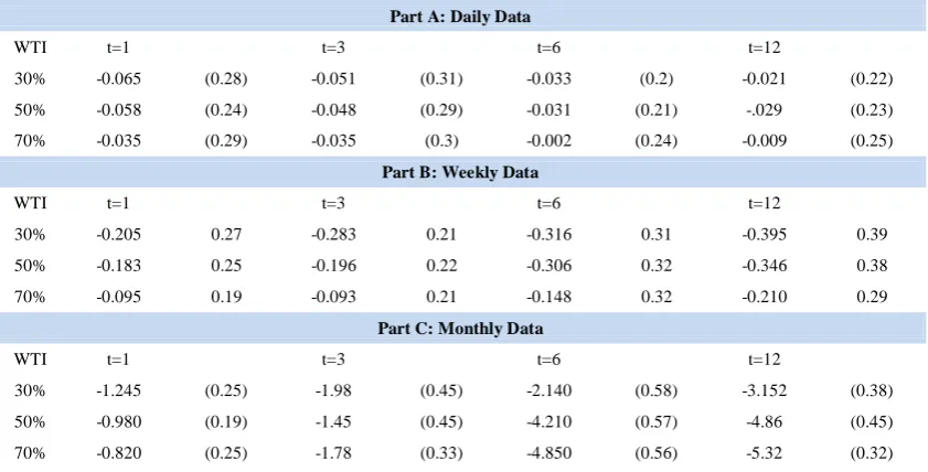
In this part we reported results which compared the OLS, ANN, and DNN predictive models based on oil price as a predictor with the historical average model as bench mark based on the daily (Part A), weekly (Part B), and monthly (Part C) data frequencies. Starting with Table 1, which presents the results of the comparison between the OLS predictive regression models to the historical average model. The table reports the statistic and the p-value of the
MSFE-adjusted statistic for assessing the statistical
significance of the corresponding forecasts under the null hypothesis that the competitor forecasts (OLS) are not better than the benchmark forecasts (historical average). Focusing on the OLS estimator results, since the statistics are negative in all cases, we found that the OLS estimator (with oil price as predictor) cannot beat the historical average model. In addition, the results are consistent across the choices of in-sample periods and forecasting horizons. We conclude that the OLS based oil price estimators are not superior to the historical average model in forecasting the stock returns.
Table 1: OLS versus historical average in stock return prediction.
Part A: Daily Data
WTI t=1 t=3 t=6 t=12
30% -0.065 (0.28) -0.051 (0.31) -0.033 (0.2) -0.021 (0.22) 50% -0.058 (0.24) -0.048 (0.29) -0.031 (0.21) -.029 (0.23) 70% -0.035 (0.29) -0.035 (0.3) -0.002 (0.24) -0.009 (0.25)
Part B: Weekly Data
WTI t=1 t=3 t=6 t=12
30% -0.205 0.27 -0.283 0.21 -0.316 0.31 -0.395 0.39 50% -0.183 0.25 -0.196 0.22 -0.306 0.32 -0.346 0.38 70% -0.095 0.19 -0.093 0.21 -0.148 0.32 -0.210 0.29
Part C: Monthly Data
WTI t=1 t=3 t=6 t=12
30% -1.245 (0.25) -1.98 (0.45) -2.140 (0.58) -3.152 (0.38) 50% -0.980 (0.19) -1.45 (0.45) -4.210 (0.57) -4.86 (0.45) 70% -0.820 (0.25) -1.78 (0.33) -4.850 (0.56) -5.32 (0.32)
Notes: This table reports the for the competitor model OLS compared to the historical average benchmark model. The in-sample proportion choices are in the first column. The DMW p-value in parentheses tests the null hypothesis 𝐻0∶ 𝑀𝑆𝐹𝐸0 ≤𝑀𝑆𝐹𝐸1 against 𝑀𝑆𝐹𝐸0>𝑀𝑆𝐹𝐸1, corresponding to
𝐻0∶ ≤0 against >0. t refers to the forecasting
horizon.
For the ANN model we observe similar result as OLS. Table 2 presents the results of the comparison between the ANN predictive models to the historical average model.
We observe the ANN model with oil price as predictors cannot beat the historical average model, since the statistics are negative in all cases. The
Table 2: ANN versus historical average in stock return prediction.
Part A: Daily Data
WTI t=1 t=3 t=6 t=12
30% -0.071 (0.13) -0.072 (0.23) -0.071 (0.19) -0.072 (0.24) 50% -0.038 (0.19) -0.036 (0.22) -0.034 (0.10) -0.032 (0.21) 70% -0.021 (0.11) -0.019 (0.17) -0.016 (0.23) -0.018 (0.22)
Part B:Weekly Data
WTI t=1 t=3 t=6 t=12
30% -0.080 (0.23) -0.082 (0.23) -0.085 (0.26) -0.083 (0.32) 50% -0.039 (0.21) -0.029 (0.22) -0.025 (0.24) -0.021 (0.27) 70% -0.023 (0.19) -0.023 (0.23) -0.019 (0.29) -0.017 (0.31)
Part C: Monthly Data
WTI t=1 t=3 t=6 t=12
30% -0.093 (0.21) -0.094 (0.25) -0.099 (0.25) -0.096 (0.25) 50% -0.041 (0.23) -0.041 (0.19) -0.036 (0.21) -0.031 (0.26) 70% -0.025 (0.22) -0.025 (0.24) -0.026 (0.18) -0.024 (0.31)
Notes: This table reports the for the competitor
model ANN compared to the historical average benchmark model. The in-sample proportion choices are in the first column. The DMW p-value in parentheses tests the null hypothesis 𝐻0∶ 𝑀𝑆𝐹𝐸0 ≤𝑀𝑆𝐹𝐸1 against 𝑀𝑆𝐹𝐸0>𝑀𝑆𝐹𝐸1, corresponding to
𝐻0∶ ≤0 against >0. t refers to the forecasting
horizon.
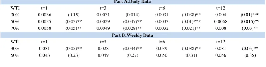
Then the DNN models with oil price as predictor was compared with the historical average model (results can be seen in Table 3). We observed that, the results are in favor of DNN models over the historical average model in forecasting stock returns. It was also observed that superiority of this model compared to historical average model is statistically significant. The results based on daily and weekly data frequencies strongly suggest that the DNN estimator is better than the historical average benchmark model, as the
takes positive values in all cases with oil price
across different in-sample periods and forecasting
horizons in the case of daily data and the ranges
from 0.0029% to 0.080% for oil price.
In the case of weekly data frequencies the
ranges from 0.018% to 0.056% for the oil price.
When monthly data were used for oil price, we obtain both positive and negative . For all forecasting horizons of 70% in-sample period the results are better than the historical average model. When daily data for oil price were consider, was statistically
significantly greater than zero at all three in sample horizon and all forecasting zone except 1 day forecasting horizon when we use 30% in-sample periods.
In the case of weekly data frequency, is
statistically significantly greater than zero when we use 30% in-sample periods and all forecasting zone and when we use 70% in sample period with 1 week forecasting horizon. For the 1 and 3 month forecast horizon and 70% in sample period for monthly data frequency is statistically significantly greater than
zero.
Table 3: DNN versus historical average in stock return prediction.
Part A:Daily Data
WTI t=1 t=3 t=6 t=12
30% 0.0036 (0.15) 0.0031 (0.014) 0.0031 (0.038)** 0.004 (0.01)*** 50% 0.0035 (0.03)** 0.0029 (0.047)** 0.0033 (0.01)*** 0.0068 (0.015)** 70% 0.0058 (0.05)** 0.0049 (0.028)** 0.0032 (0.021)** 0.008 (0.03)**
Part B:Weekly Data
WTI t=1 t=3 t=6 t=12
70% 0.018 (0.049)** 0.032 (0.38) 0.044 (0.21) 0.048 (0.26)
Part C:Monthly Data
WTI t=1 t=3 t=6 t=12
30% -0.19571 (0.35) -1.62215 (0.32) -0.21611 (0.4) -0.21525 (0.22) 50% -1.50148 (0.2) -1.51147 (0.3) -1.44711 (0.37) -1.3365 (0.45) 70% 0.049201 (0.078)* 0.049223 (0.05)** 0.054119 (0.24) 0.055296 (0.21)
Notes: This table reports the for the competitor
model DNN compared to the historical average benchmark model. The in-sample proportion choices are in the first column. The DMW p-value in parentheses tests the null hypothesis 𝐻0∶ 𝑀𝑆𝐹𝐸0 ≤𝑀𝑆𝐹𝐸1 against 𝑀𝑆𝐹𝐸0>𝑀𝑆𝐹𝐸1, corresponding to
𝐻0∶ ≤0 against >0. t refers to the forecasting horizon. *, **, *** denote significance at the 10%, 5% and 1% levels, respectively
4.2. Economic significance
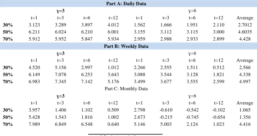
Utility gains at risk aversion factors of three and six were calculated and besides that results at all four different forecasting horizons as defined in the previous section were reported.
It was observed that the DNN model provides a more precise stock return forecasting than the historical average model. Therefore, the utility gains are expected to be positive and the results clearly support this expectation. Utility gains obtained from the DNN model instead of the historical average for stock returns forecast are reported in Table 4.
It was found that utility gains at all forecasting horizons and using both three and six risk aversion factors are positive for daily and weekly data frequencies. In the case of monthly frequency, when we use a risk aversion factor equal to three the utility gains are positive. Our results suggest that mean-variance investors are able to obtain utility gains by using the DNN instead of the historical average model. The results are robust across the in-sample periods, risk aversion parameters and forecasting horizons. Another significant fact is that the positive utility gains are fairly sizeable. Considering the daily data results, the utility gains vary in a range from 1.562% to 6.211 %, and the average value is 3.9 %. This result can be interpreted as an investor being willing to pay an extra 3.9% per annum to have access to the additional information available in the DNN predictive approach. The results are similarly based on weekly and monthly data models, where the average utility gains over in-sample periods risk aversions and forecasting horizons are 2.2% and 3.9%, respectively.
Table 4: Utility gains from using the DNN instead of historical average
Part A: Daily Data
ɣ=3 ɣ=6
t=1 t=3 t=6 t=12 t=1 t=3 t=6 t=12 Average
30% 3.123 3.289 3.897 4.012 1.562 1.666 1.951 2.110 2.7012
50% 6.211 6.024 6.210 6.001 3.155 3.112 3.115 3.000 4.6035
70% 5.912 5.952 5.847 5.934 2.959 2.988 2.933 2.899 4.428
Part B: Weekly Data
ɣ=3 ɣ=6
t=1 t=3 t=6 t=12 t=1 t=3 t=6 t=12 Average
30% 4.520 5.156 2.997 1.012 2.266 2.555 1.511 0.512 2.566
50% 6.149 7.078 6.253 3.643 3.088 3.544 3.128 1.821 4.338
70% 6.983 7.345 7.142 5.176 3.499 3.677 3.555 2.599 4.997 Part C: Monthly Data
ɣ=3 ɣ=6
t=1 t=3 t=6 t=12 t=1 t=3 t=6 t=12 Average
30% 3.957 1.406 1.102 0.509 2.798 -0.610 -0.542 -0.102 1.065
50% 5.428 1.543 1.816 1.002 2.673 -0.215 -0.745 -0.654 1.356
Notes: This table reports the average utility gains of using the DNN model based on the oil price instead of the historical average model to forecast the stock returns. The in-sample proportion choices are in the first column. t refers to the forecasting horizons and 𝛾 refers to the risk-aversion.
5. Discussion and Conclusions
This paper has used S&P500 indices crude oil price for stock returns forecast. It has used DNN forecasting model, which has solved some problems related to ANN model such as gradient vanishing and randomly weighted matrix. Due to DNN structure and it’s sensitively to the number of data, daily, weekly and monthly data has been used over the period from 4 January 1986 to 31 December 2017 to find out the effect of data frequencies on the model prediction ability. Three choices of in-sample periods with the proportions of 30%, 50% and 70% of the full sample were utilized for data mining and to overcome the over fitting in order to predict the out-of-sample stock returns. The practical analyses were repeated with a different oil price series to test the robustness of the results.
The main findings and offerings of this research are: First, unlike the existing literature on oil price and stock returns, it has focused on out-of-sample prediction of returns. It has showed that the estimator has a great role and how well the oil price forecasts stock returns does not only depend on the data frequency but it also relies on the estimator. Pair-wise assessments has been employed between the OLS, ANN and DNN models with historical average benchmark model. It has been observed that the DNN model using performs better than the historical average model in forecasting stock returns when the crude oil price is used as a predictor. This has been opposite for the OLS and ANN models. The outperformance of the DNN over the other models is data frequency-dependent. It is strongly evident in the daily and weekly data frequencies and it is found to be weaker when monthly data has been used.
6. Acknowledgment
Sabbatical financial support provided by Kermanshah branch of Islamic Azad University is appreciated.
References
1) Adebiyi, A., Adewumi, A., Ayo, C. (2014). Comparison of ARIMA and artificial neural networks models for stock price prediction. Journal of Applied Mathematics, Available on internet at http://dx.doi.org/10.1155/2014/614342 article_id= 614342.
2) Agrawal, J., Chourasia, V., Mittra, A. (2013). State-of-the-art in stock prediction techniques. International Journal of Advanced Research in Electrical, Electronics and Instrumentation Engineering, 2 (4), 1360–1366.
3) Ahmadi, E., Jasemi, M., Monplaisir, L., Nabavi, M., Mahmoodi., A., Amini Jam, P. (2018). New efficient hybrid candlestick technical analysis model for stock market timing on the basis of the support vector machine and heuristic algorithms of imperialist competition and genetic. Expert Systems with Applications, 94 (1), 21-31. 4) Ang, A., Bekaert, G. (2007). Stock return
predictability: Is it there? Review of Financial studies, 20 (3), 651–707.
5) Bishop, C., M. (2006). Pattern Recognition and machine learning. Springer, Germany.
6) Brooks, C. (2015). Introductory econometrics for finance. 3rd ed., Cambridge university press, 419- 424.
7) Bollerslev, T., Marrone, J., Xu, L., Zhou, H. (2014). Stock return predictability and variance risk premia: Statistical inference and international evidence. Journal of Financial and Quantitative Analysis, 49 (03), 633–661.
8) Brennan, M., Xia, Y. (2005). Tay’s as good as cay. Finance Research Letter, 2, 1-14.
9) Brock, W., Lakonishok, J., Lebaron, B. (1992). Simple technical trading rules and the stochastic properties of stock returns. The Journal of Finance, 47, 1731-1764.
10) Butler, A., Grullon, G., Weston, J. (2005). Can managers forecast aggregate market return? Journal of Finance, 60, 963-986.
11) Campbell, S. D. (2012). Macroeconomic
volatility, predictability, and uncertainty in the great moderation. Journal of Business and Economic Statistics, 25(2), 191-200.
12) Campbell, J., Thompson, S. (2008). Predicting excess stock returns out of sample: Can anything beat the historical average? Review of Financial Studies, 21 (4), 1509–1531.
14) Clark, T., West, K. (2007). Approximately normal tests for equal predictive accuracy in nested models. Journal of Econometrics, 138, 291-311. 15) Diebold, F., Mariano, R. (1995). Comparing
predictive accuracy. Journal of Business and Economic Statistics, 13, 253-263.
16) Driesprong, G., Jacobsen B., Maat, B. (2008). Striking oil: Another puzzle? Journal of Financial Economics, 89, 307-327.
17) Ferreira, M., Santa-Clara, P. (2011). Forecasting stock market returns: The sum of the parts is more than the whole. Journal of Financial Economics, 100 (3), 514–537.
18) Goyal, A., Welch, I. (2008). A comprehensive look at the empirical performance of equity premium prediction. Review of Financial Studies, 21(4), 1455-1508.
19) Goyal, A., Welch, I. (2003). Predicting the equity premium with dividend ratios. Management Science, 49, 639-654.
20) Hamilton, J. D. (1983): Oil and the Macro Economy since World War II. Journal of Political Economy, 91: 228-248.
21) Jasemi, M., Kimiagari, A., Memariani, A. (2011a). A conceptual model for portfolio management sensitive to mass psychology of market. International Journal of Industrial Engineering Theory Application and Practice, 18 (1), 1–15.
22) Kim, Y., Enke, D. (2016a). Developing a rule change trading system for the futures market using rough set analysis. Expert Systems with Applications, 59, 165–173.
23) Kim, Y., Enke, D. (2016b). Using neural networks to forecast volatility for an asset allocation strategy based on the target volatility. Procedia Computer Science, 95, 281–286. 24) Kim, J., Shamsuddin, A., Lim, K., (2011). Stock
return predictability and the adaptive markets hypothesis: Evidence from century-long us data. Journal of Empirical Finance, 18 (5), 868–879. 25) Kong, A., Rapach, D., Strauss, J., Zhou, G.
(2011). Predicting market components out of sample: asset allocation implications. Journal of Portfolio Management 37, 29-41.
26) Lee, C., Sehwan, Y., Jongdae, J. (2007). Neural Network model versus ARIMA model in forecasting Korean stock price index. Information System, 8 (2), 372–378.
27) Lee, K., Chi, A., Yoo, S., Jin, J. (2008). Forecasting Korean stock price index using back propagation neural network model, bayesian chiao’s model, and ARIMA model. Academy of Information and Management Sciences Journal, 11 (2), 53 -75.
28) Miller, J., Ratti, R. (2009). Crude oil and stock markets: Stability, instability and bubbles. Energy Economics, 31, 559-568.
29) Nair, V., Hinton, G., (2010): Rectified linear units improve restricted Boltzmann machines. 27th international conference on machine learning, 807–814.
30) Narayan, P., Amhed, H., Narayan, S. (2015). Do momentum-based trading strategies work in the commodity futures markets? Journal of Futures Markets, DOI: 10.1002/fut.21685.
31) Narayan, P., Narayan, S., Sharma, S. (2013). An analysis of commodity markets: What gain for investors? Journal of Banking and Finance, 37, 3878-3889.
32) Narayan, P., Narayan, S. (2010). Modelling the impact of oil prices on Vietnam's stock prices. Applied Energy, 87, 356-361.
33) Narayan, P., Sharma, S., Poon, W, Westerlund, J. (2014). Do oil prices predict economic growth? New global evidence. Energy Economics, 41, 137-146.
34) Narayan, P., Sharma, S. (2011). New evidence on oil price and stock returns. Journal of Banking and Finance, 35, 3253-3262.
35) Pettenuzzo, D., Timmermann, A., Valkanov, R. (2014). Forecasting stock returns under economic constraints. Journal of Financial Economics, 144 (3), 517–553.
36) Park, J., Ratti, R. (2008). Oil price shocks and stock markets in the U.S. and 13 European countries. Energy Economics, 30, 2587-2608. 37) Phan, D., Sharma, S., Narayan, P. (2015). Stock
return forecasting: Some new evidence. International Review of Financial Analysis, 40, 38–51. E.
38) Rapach, D., Strauss, J., Zhou, G. (2010). Out-of-sample equity premium prediction: Combination forecast and links to the real economy. Review of Financial Studies, 23, 821-862.
39) Rather, A., Sastry, V., Agarwal, A. (2017). Stock market prediction and Portfolio selection models: a survey. OPSEARCH, 54, 558-579.
40) Soytas, U., Sari, R., Hammoudeh, S.,
Hacihasanoglu, E. (2009). World oil prices, precious metal prices and macro economy in turkey. Energy Policy, 37(12), 5557–5566 41) Tashman, L. (2000). Out-of-sample tests of
forecasting accuracy: an analysis and review. International Journal of Forecasting, 16, 437-450. 42) Wei C. (2003). Energy, the stock market and the
Putty-Clay investment model. American
Economic Review, 93, 311–23.
premium prediction. Review of Financial Studies, 21, 1455-1508.
44) West, K. (1996). Asymptotic inference about predictive ability. Econometrica, 64, 1067-1084. 45) Westerlund, J., Narayan, P. (2012). Does the
choice of estimator matter when forecasting stock returns. Journal of Banking and Finance, 36, 2632-2640.
Notes
1
See Goyal and Welsh, 2008.
2
Economic variable like: consumption-wealth ratio (Lettau and Ludvigson, 2001), inflation rate (Nelson, 1976; Fama and Schwert, 1977), nominal interest rates (Breen et al., 1989) and price ratio (Fama and French, 1988, 1989).
3
Financialvariables like: book-to-market ratio (Kothari and Shanken, 1997; Pontiff and Schall, 1998), corporate issuing activity (Baker and Wurgler, 2000), dividend, earnings-price ratio (Campbell and Shiller, 1988), term and default spreads (Campbell, 1987; Fama and French, 1989).
4
For more discussion on this issue see Narayan and Sharma (2015).
5
See Narayan and Sharma (2015).
6 Data preprocessing or data representation is the first level in
machine learning algorithm and before model estimated this problem had been solved by feature engineering.
7
This test statistic is now widely used in the applied time series forecasting literature (see Rapach et al., 2010 and Kong et al., 2011).
8 In other words, an investor will invest more in the risky