IMPROVED OPTION PRICING USING ARTIFICIAL NEURAL NETWORKS AND BOOTSTRAP METHODS

c

World Scientific Publishing Company

IMPROVED OPTION PRICING USING

ARTIFICIAL NEURAL NETWORKS AND BOOTSTRAP METHODS

PAUL R. LAJBCYGIER∗

School of Business Systems, Monash University, Clayton, Victoria, Australia 3168

JEROME T. CONNOR†

London Business School, Sussex Place, Regents Park, London NW1 4SA, UK

Ahybridneural network is used to predict the difference between the conventional option-pricing model and observed intraday option prices for stock index option futures. Confidence intervals derived with bootstrap methods are used in a trading strategy that only allows trades outside the estimated range

of spurious model fits to be executed. Whilsthybridneural network option pricing models can improve

predictions they have bias. The hybrid option-pricing bias can be reduced with bootstrap methods. A modified bootstrap predictor is indexed by a parameter that allows the predictor to range from a pure bootstrap predictor, to a hybrid predictor, and finally the bagging predictor. The modified bootstrap predictor outperforms the hybrid and bagging predictors. Greatly improved performance was observed on the boundary of the training set and where only sparse training data exists. Finally, bootstrap bias estimates were studied.

1. Introduction

Conventional option-pricing modeling is founded on the seminal work of (Black and Scholes, 1973). Claims that the Black-Scholes valuation model no longer holds are appearing with increasing and alarming frequency (Dumas et al., 1996; Bates, 1997a). Persistent, systematic and significant option pricing biases exist. This work is concerned with im-proving the option-pricing accuracy of the conven-tional option-pricing approach.

The failure of the conventional model has mo-tivated a new ‘modern’ option pricing literature de-termined to reconcile these option-pricing anomalies. Researchers have explored a number of directions.

The underlying assumptions of the Black-Scholes model have been systematically generalised. Extend-ing conventional analytical approaches by incorpo-rating stochastic option pricing parameters (other than underlying returns) has been a natural place to begin (Hull and White, 1987; Johnson and Shanno, 1987; Ball, 1994). Considering market frictions (such

as transaction costs) has also been explored. Whilst generalising the underlying assumptions is obvious it often leads to intractable mathematics and compli-cated parameter estimation. In fact, (Bates, 1997b) claims that “most postulated processes can be ruled outa priorias inconsistent with observed. . .biases.” These difficulties have motivated different direc-tions. When developing their model (Black and Scholes, 1973) knew that price return distributions were not lognormal, however they decided to use this assumption for the sake of analytical tractability. Option-pricing theory permits the estimation of the underlying distribution. This can be used to price options in a very intuitive manner. However, the approach has its problems. A prior distribution is required (Rubinstein, 1994). The empirical underly-ing distribution can only have positive probabilities. The tails of the distribution can be difficult to es-timate due to sparse data. The method has been shown not to work well out-of-sample (Dumaset al., 1996). Market practitioners often think in terms of

∗_{E-mail: [email protected]} †_{E-mail: [email protected]}

implied volatility. Therefore, modeling the implied volatility is another intuitive approach (Ncube, 1996; Dermanet al., 1996; Heynen, 1994a; Ait-Sahalia and Lo, 1995). Whilst intuitive, the approach often as-sumes that the volatility is stationary. In general, this is not true.

Those approaches that hold the most promise are those which are simplest and make minimal as-sumptions. The hybrid approach is one such ap-proach. The hybrid option pricing approach pre-dicts the residuals between conventional model price and actual transaction price using an artificial neural network (ANN). These residual predictions are used to augment the optimal conventional option-pricing model out-of-sample. This work shows that sta-tistically and economically significant out-of-sample pricing performance is possible using the hybrid neural network approach.

Re-sampling techniques are used to:

• estimate hybrid confidence limits which identify profitable trading strategies;

• consider methods of bias reduction by using a novel combination of bootstrap and bagging;

• study the quality of the hybrid model by estimat-ing hybrid model bias as a function of option input parameters.

A number of similar approaches have been at-tempted. The most similar is (Gultekinet al., 1982), who modeled the residuals with linear regression for Chicago Board Options Exchange (CBOE) call op-tions during 1975–1976. They found statistically sig-nificant out-performance when modeling the residu-als. More recently, (Jacquier and Jarrow, 1996) used a Bayesian approach for modeling the residuals for options transacted on the US share Toys R Us from December 1989 to 1994. They found that the Black-Scholes model performed well after taking into ac-count model specification errors.

This paper is organised into six sections. Section 2 provides all the necessary finance required for an understanding of the work. Section 3 intro-duces the hybrid neural network approach. Section 4 utilizes bootstrap confidence limits in static op-tion trading strategies. Secop-tion 5 introduces a novel mixture of bootstrap and bagging to minimize model bias. Finally, Sec. 6 examines the bias of the hybrid model as a function of the option-input parameters.

2. Finance Background

2.1. Futures and options

A futures contract is an obligation to either buy or sell a specific commodity — known as the underly-ing— at an agreed price at some time in the future. Futures have an expiry time. At expiry the holder of the future must either buy or sell the underlying at the price specified in the futures contract. The futures market is a no net gain market. For each investment there will always be an equal and op-posite investment. This implies that for every dol-lar that one investor makes, another investor, who took the opposite trade makes an equal and opposite loss.

Stock market indices are designed to reflect over-all movements in a large number of equity (i.e. share) securities. The performance of an equity index is im-portant because it represents the performance of a broadly diversified stock portfolio and gives insights into the broad market risk/return profile.

Index futures are contracts that commit the user to either buy (go long) or sell (go short) the stocks in the index at the currently determined market price at some point in the future. If the investor believes the index to be going down he shouldsell/go short. If, on the other hand, the investor believes that the index is going up he shouldbuy/go long.

exercised. An option on a future is the right but not the obligation to purchase the future at the strike price before the expiry.

One final distinction is between American and European style options. Americanstyle options can be exercised at any time prior to expiration, whilst European style options can only be exercised at expiry.

2.2. The Australian options on futures market

Stock market indices are designed to reflect the over-all movement in a broadly diversified equity port-folio. The Australian Stock Exchange (ASX) All Ordinaries Share Price Index (SPI) is calculated daily and represents a market value weighted index of firms that consist of over 95% by value all firms cur-rently listed on the ASX. A future written on the SPI is traded on the Sydney Futures Exchange (SFE). The SFE is the world’s ninth largest futures market and the largest non-computer traded market in the Asia-Pacific region. The 1995 average daily volume for SPI futures was 9,795 contracts.

The SPI futures option is written on the SPI futures contract. Exercise prices are set at intervals of 25 SPI points. Options expire at the close on the last day of trading in the underlying futures and may be exercised on any business day prior to and includ-ing expiration day. Upon exercise, the holder of the option obtains a future’s position in the underlying future at a price equal to the exercise price of the option. When the future is marked to market at the close of trading on the exercise day the option holder is able to withdraw any excess. To give an indication of liquidity, in 1995 there were, on average, 3,100 SPI options on futures contracts traded daily.

The role of theclearing-houseis to guarantee that investors can meet their trading obligations. A sys-tem of cash deposits known asmarginsis used by the clearing house to guarantee that traders can meet their obligations.

The SFE is peculiar in that both the option writer and the option buyer must post a margin with the clearing-house. The option buyer does not have to

pay a full premium to the writer. Instead, a portion of the premium from both the buyer and the writer is deposited with the house. The clearing-house provides the writer with credit for any market move in his favor and vice versa. The full premium may not be given to the writer until the option is exercised or expires (Martini and Taylor, 1995).

2.3. Conventional option pricing for the SFE

(Black and Scholes, 1973) created parametric models to price call options using the assumption that the underlying follows a random diffusion process.

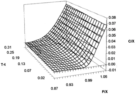
The SFE uses a system of deposits and margins for both long and short option positions which re-quires a modification of the standard diffusion pro-cess, see (Martini, 1995). This modification reflects the fact that no interest can be earned on a premium that has not been paid fully up front. Essentially the interest rate, r is set to zero in the Black solution. The relative option price or premium,C/X,ais given by the modified Black model as

fM B(x) = (F/X)N(d1)−N(d2) (1)

where d1 = (In(F/X) + (σ2/2)(T −t))/σ

√

T−t, d2=d1−σ

√

T−t,F is the underlying futures price,

T −t is the time to maturity (in years), σ is the

Fig. 1. The modified Black option-pricing surface.

a_{The use ofF /XandC/X in place ofF,X andChas been used see (Hutchinsonet al., 1994) and (Merton, 1973). Although the}

standard deviation of the underlying, (·) is the stan-dard normal cummulative distribution function, and the set of inputs are denoted byx= (F/X, T−t, σ).

The modified Black pricing surface is shown in Fig. 1. The modified Black model is the accepted standard at the Sydney Futures Exchange; all mar-gin requirements imposed by the exchange are de-rived from it.

2.4. Weighted implied standard deviation

Only one option pricing parameter is not known ex-actly prior to option transaction time — the stan-dard deviation, σ. Prior to the option transaction this cannot be known, an estimate is required.

After the transaction, it is possible to determine the standard deviation implied (ISD) by the option transaction price.b

There are a number of ways of obtaining an esti-mate of the standard deviation:

• model the ISD using a time seriesc _approach.

• choose the standard deviation that minimizes the option pricing error from previous transactions.d

• calculate a weighted average of ISDs from previous transactions — Weighted Implied Standard Devi-ation (WISD).

WISD’s are considered the optimal standard devia-tion estimadevia-tion approach in this work.

It is possible to consider any individual ISD as consisting of:

• primarily, the market’s realized standard deviation predictione

• less significantly, a combination of bias (due to moneynessandmaturity)f

• noise (due, for example, to bid-ask spread, sup-ply/demand).

The reason that WISD’s are considered the optimal standard deviation approach is because they can mit-igate the option pricing biases, minimize the effect of noiseg _{and therefore obtain the most accurate} esti-mate of the markets standard deviation.

(Figlewski, 1997) has criticized the use of WISD’s. He argues that suppressing ISD differences across different options by an averaging process can-not be appropriate when systematic and persistent option pricing biases exist. Figlewski argues that the biases imply that the market is using a different option-pricing model.

Consistent with Figlewski’s argument a new option-pricing model is estimated in this work (see Sec. 3). Nevertheless, an estimate of standard de-viation is required. Although WISDs provide the optimal standard deviation estimation approach, it is not clear which WISD in particular is best. There are three separate requirements which determine the choice of optimal WISD. The first is that the choice of WISD must be one that minimizes option-pricing error.h_{The second is that the WISD provides}

b_{The implied standard deviation (ISD) of options on futures contracts is defined as the standard deviation which equates the}

modified-Black model price with the observed option price given (C/X, T−t, F /X).

c_{It is also possible to forecast future market implied volatility using time series models. In this work, a WISD approach is preferred}

to a time series approach for the forecasting of standard deviation, for numerous reasons: First, the AO SPI options on futures are reasonably illiquid, so few transactions are available to model ISD; second, strong hourly auto-correlation and mean reversion has been noted on illiquid option markets such as the Spanish IBEX 35 by (Refenes and Miranda, 1996) and on the Paris stock exchange by (Jacquillantet al., 1993). In such markets liquidity is thin and buy/sell imbalances have an accentuated effect. Finally, (Roll, 1984) has shown that that because each transaction must take place at either the bid or the ask level, random movements between the bid-ask–‘bid-ask bounce’ cause significant negative serial correlation. Nevertheless, previous work has attempted not only to make comparisons between historical standard deviation time series modeling (Park and Sears, 1985) but also to model the ISD using various time series techniques (Christensen and Prabhala, 1994; Diz and Finucane, 1993; Refenes and Miranda, 1996; Engle and Mustafa, 1992).

d_{(Martini and Taylor, 1994) show that this approach cannot work for the SFE options data because there are not enough valid}

transactions.

e_{The underlying’s realized stardard deviation is the standard deviation calculated over the life of the option.}

f_{The moneyness and maturity biases refer to the empirical fact that there exist persistent and systematic biases which are a function}

of the ratio of the underlying price/strike price and time to maturity of the option respectively.

g_{(Figlewski, 1997) argues that the bid-ask spread can have a large effect on ISD. Furthermore, he argues that WISD’s mitigate}

bid-ask spread effects due to the consideration of options on both the bid and ask side of the spread used in the averaging process.

h_{“. . .the implied volatility need have little to do with the best possible prediction for the price variability of the underlying asset}

from the present through option expiration, while it has everything to do with the current and near term supply and demand. . . .” (Figlewski, 1997)

i_{It is possible to apply arbitrage arguments, which imply that they must be identical. (Figlewski, 1997) argues that arbitrage}

an accurate predictor of realized underlying stan-dard deviation.i _{Finally, we desire that the WISD} must be a plausible predictor of realized standard deviation.j

Those WISDs that weighat-the-moneyISDs most heavily fulfil each of the above requirements. Those WISD schemes which give more weight to at-the-moneyoptions tend to be the most accurate for price prediction. The reasons for this accuracy are that these options trade with much greater liquidity than others and therefore their ISD’s contain more reliable information; also,at-the-moneyoption premiums are most sensitive to changes in the standard deviation (Figlewski, 1997). Previous studies which show that at-the-money WISD’s are optimal for price predic-tion include (Turvey, 1990) and (Martini and Taylor, 1994).

Those WISD schemes that give more weight to at-the-money options tend to be the most accu-rate for realized standard deviation prediction too. (Corrado and Miller, 1996a) prove theoretically that at-the-moneyWISD’s are the most efficient (and also ‘nearly’ unbiased) predictors of realized standard de-viation. This is verified by various empirical studies (Canina and Figlewski, 1993; Chiras and Manaster, 1978).

Finally, at-the-money WISDs provide plausible realized standard deviation estimates. This is not true of WISDs which use ISD estimates from those

transactions which are have the most similar money-ness to the one under consideration. These WISD’s provide non-unique realized standard deviation esti-mates. Therefore, this type of WISD is not a plau-sible predictor of realized standard deviation.

A number of WISD’s are compared empirically in (Lajbcygier, 1998). Not surprisingly it is shown that anat-the-moneyWISD–DERISD, is the optimal WISD. DERISD = ˆσimp = (

PK

i=1σ 2 imp,iΛ

2 imp,i)

1/2 /

(PKi=1Λ 2 imp,i)

1/2

and σimp,i are the ISD’s from K previous same dayk _{options and Λ = ∂f}

M B(x)/∂σ (i.e. the sensitivity of the option price with respect to the standard deviation). Same day intraday trans-action data are used for the calculation of the WISD.l The input vector used in Eqs. (1), (2) and the rest of this paper is changed to reflect this estimated data tox= (F/X, T−t,σˆDerisd).

3. The Hybrid-Artificial Neural Network Approach

Motivated by the good initial fit to the data pro-vided by the modified Black model, we use ahybrid approach in which non-parametric regression tech-niques model the residuals between the option trans-action prices and the modified Black model prices.

The fundamental advantage of non-parametric regression is that it makes very few assumptions about the unknown function to be estimated.

j_{The (Black and Scholes, 1973) model assumes constant standard deviation. This cannot be known a priori, a forecast must be}

made. Either historical standard deviation, implied standard deviation (ISD) or a combination of both must be used to provide a forecast. Historical standard deviation is calculated using an arbitrary rolling window of the log returns of the underlying. ISD is defined as the standard deviation that equates the conventional model price with the observed model price. The ‘pricing ISD hypothesis’ states that the ISD is a better predictor of option price than historical standard deviation. This is supported by most empirical studies. The ‘realized ISD hypothesis’ states that ISD is a better predictor of realized standard deviation than historical standard deviation. This hypothesis is not supported clearly by the empirical option pricing literature. The early literature found ISD to be better at forecasting future standard deviation (Latane and Rendleman, 1976; Chiras and Manaster, 1978). However, (Canina and Figlewski, 1993) found evidence against the hypothesis for S&P 100 options (although additional research by (Geske and Kim, 1994) and (Christensen and Prabhala, 1994) cast doubts on (Canina and Figlewski, 1993) results). (Day and Lewis, 1992a), (Fleminget al., 1995), (Jorion, 1995), (Xu and Taylor, 1995) and (Guo, 1996) all provide evidence in favor of the hypothesis. Overall the empirical literature supports the ISD hypothesis. Therefore, in this paper, we also use ISD. However, due to this ambiguity historical volatility has also been considered elsewhere (Lajbcygier, 1998).

k_{Others have suggested the use of intraday data. (Figlewski, 1997) states that it is possible to “extract(ing) more information from}

a set of option prices by averaging across multiple intraday observations on the same options, in order to reduce the impact of price noise from the bid-ask spread,” (Brenner and Galai, 1981) also found that additional forecasting power can be achieved by calculating WISD’s intraday. We are not aware of any other study which utilizes same day WISD. There are strong intuitive reasons for using the same day ISDs to calculate WISDs. Firstly, overnight effects in overseas markets can be quite large. Secondly, it seems sensible to use the most up-to-date ISD estimate rather than to rely on the previous days. Finally,T−twill be exactly the same for each option since the options are separated by maturity date — this would not be the case if the previous day’s options were used.

l_{In principle bid-ask spread mid-point prices should be used and not transaction prices as in this study. However, as (Figlewski,}

(Lajbcygier and Flitman, 1996) has compared ar-tificial neural networks (ANN’s) with a method from each of the general classes of non-parametric regression methods: global parametric methods (i.e. linear regression), local parametric methods (i.e. kernel regression) and adaptive computation methods (i.e. projection pursuit regression). ANN’s were among the most accurate regression techniques compared.

The relationship between the option input variables (i.e.F/X, T −tm_,σn

Derisd) and the resid-uals shows that there are persistent and systematic (weakly) nonlinear biases. Furthermore, weak inter-actions between the input variables are shown to ex-ist. ANN’s are eminently suitable for modeling such functions.

The hybrid model can be depicted mathemati-cally as follows:

fhybrid(x) =fM B(x)−fN N(x). (2)

Hybrid neural networks of the form in Eq. (2) were shown to outperform hybrid linear models, for a sim-ilar data set, by a factor of two in (Lajbcygier and Flitman, 1996a).o

Intraday call option transactions were considered from Jan 1993 to December 1993. The first half of

the data, January through June, was used as an esti-mation set and the rest was reserved for out of sample testing.

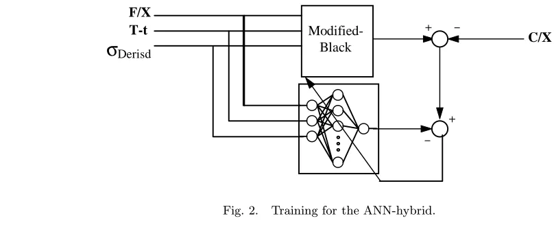
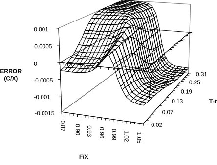
A three layer, fifteen hidden unit neural network was estimated using backpropagation with a 20% cross validation set used for network selection. What follows is an analysis of the ANN-hybrid output. The estimated hybrid option-pricing model is shown in Fig. 3–5. They plot the output of the Modified Black hybrid ANN as a function ofF/X andT−t.

Figure 3 is the ANN output surface for the standard deviation equal to 0.11 — the lowest standard devi-ation for the in-sample data, while Fig. 5 is the same surface for standard deviation equal to 0.28 — the highest standard deviation in the in-sample set.

In general, the surfaces are complicated, smooth and imply consistent mis-pricings in the conventional models of between 2 and−2 points (approximately $50 and −$50 per option respectively, if we assume a strike ofX = 2000).

The most striking feature of the hybrid ANN output at all standard deviations is the ridge at

F/X ≈ 1. This divides the options into those that have positive and negative value relative to the con-ventional option-pricing model (see Table 1).

This is consistent with both the (Rubinstein, 1994) and (Derman and Kani, 1994) studies of

F/X

C/X

Modified-Black

T-t

σ

-+

+

-Fig. 2. Training for the ANN-hybrid.

m_{In this paper, to mitigate maturity bias, the options were classed by time to maturity. Different implied volatilities were calculated}

for different times to maturity. Weightedσimp’s are calculated only from options transacted on the same day.

n_{It was decided to extract the nearest recent SPI futures price that was recorded before the time that the option was transacted.}

This resulted in underlying values that in most cases were recorded only seconds before the option was transacted. If the underlying future was transacted more than 60 seconds prior to the option, the option transaction was discarded.

o_{When using a neural network on its own to model a call option there exists considerable discrepancy from the conventional model}

Table 1. Positive (+) value above conventional model, (−) value below conventional model. Short Maturity (0–0.15) Long Maturity (0.15–0.3)

In the Money (0.9–1) + +

Out of the Money (1–1.1) +/− −

Fig. 3. Hybrid ANN output, standard deviation

σ= 0.11.

0.02 0.07

0.13 0.19

0.25 0.31

-0.0015 -0.001 -0.0005 0 0.0005 0.001

ERROR (C/X)

F/X

T-t

0.

96

0.

87 0.

90 0.93 0. 99 1.02 1.₀₅

Fig. 4. Hybrid ANN output, standard deviation

σ= 0.2.

the S&P 500 CBOE futures options. (Rubinstein, 1994) conjectures that this bias is caused by in-vestors’ fear of a repeat of the 1987 crash. The shape of the hybrid surface is almost identical to the devi-ations noted by (Corrado and Miller, 1996a) for the S&P 500. This is quite remarkable given the different markets.

0.02 0.07

0.13 0.19

0.25 0.31

-0.0015 -0.001 -0.0005 0 0.0005 0.001

0.

96

0.

87 0.

90 0.93 0.₉₉ 1. 02 1.05

ERROR (C/X)

T-t

F/X

Fig. 5. Hybrid ANN output, standard deviation

σ= 0.28.

For low standard deviation (see Fig. 3), out of the money short time to maturity options are valued more highly than the conventional model. This low standard deviation effect has not been emphasized in prior studies.

It is interesting to compare and contrast Fig. 3 and Fig. 5 to ascertain the interaction between the surface variables: F/X andT −t,and σ. No large differences in the surfaces exist, but there are five subtle changes. Firstly, the top flat region in Fig. 3 has extended and moved forward. Secondly, the top flat region in Fig. 3 has shifted up. Thirdly, the bot-tom of the surface nearT−tequal to zero has moved up. Fourthly, the region between the flat top and the steep wall on the right of the surface is smoother. Finally, the dip atF/Xequal to 1.02 andT−tequal to 0.07 in Fig. 3 has become shallower in Fig. 5.

4. Trading Strategies Based on Bootstrap Confidence Intervals

Fig. 6. Out-of-the-moneyoption price premium versusF/X: The Modified Black pricing model falls within the confidence

intervals of the “hybrid” model. The option pricing parameters areT−t= 0.1, σ= 0.15, X= 2000.

Fig. 7. At-the-money option price premium versus F/X: In some regions such as F/X = 0.98 the two models are

option pricing models and deciding when a trade should be executed.

Due to neural networks nonlinearity and struc-tural complexity, classical statistical theory pro-vides little help in estimating confidence limits. (Chryssolouris, 1996) requires unrealistic and strong assumptions (i.e. normal errors) to estimate confi-dence limits for neural networks.

In this work, confidence intervals for option pric-ing models are generated by bootstrap methods. For an introduction to bootstrap methods see (Efron and Tibshirani, 1993) or in the context of neural networks see (Tibshirani, 1996), (LeBaron and Weigend, 1998) or (Pass, 1993).

Given a total ofnoptions in the data-set,i boot-strap data sets are generated. Bootboot-strap data sets

Li = {(c (i)

j ,xj), j = 1, . . . , n} are generated by

c(_ji) = ˆfhybrid(x) +e (i)

j where e (i)

j are drawn ran-domly with replacement from the empirical distri-bution p(e) = n−1P

iδ(e − ˆei), and ˆei are the observed residuals from initial hybrid model fit. This is known as a “bootstrap residual approach” (Tibshirani, 1996).p _{Predictors, ˆf}(i)_{(x), are} esti-mated on the bootstrap data sets, Li, in the same manner as the hybrid predictor. The bootstrap as-sumption for confidence intervals is

(f(x)−fˆhybrid(x))2≈ 1

N−1 N

X

i=1

( ˆfhybrid(x)−fˆ(i)(x))2

(3) where f(x) is the true function, andN is the num-ber of bootstrap data series simulated, in this case 30. (Tibshirani, 1996) usedN = 20,he argues this is a lower limit on the number of bootstrap replications but necessary due to the complicated ANN model. In Fig. 6, confidence intervals computed in (3) and cen-tred at the hybrid predictor are shown for +/−one standard deviation. Bootstrap and bagging predic-tors are also plotted in Fig. 6 and will be discussed in Sec. 5. The width of the confidence intervals varies over the input space. In the region ofat-the-money options, Fig. 7 confidence intervals are much tighter than for deep out of the money options. The

modi-fied Black predictor often falls outside the confidence intervals. In these regions, confidence can be placed in the hybrid predictors.

Bootstrap confidence intervals allow the identifi-cation of option prices, which both appear profitable and are outside the range of model uncertainty. Since the confidence intervals vary over the input space of the model trading positions will be confined to areas of greater certainty.

Identification of profitable tradesq_{is not the only} use for better option pricing models. The process of limiting exposure of a financial position to changes in underlying assets is known as hedging and is de-termined by the option pricing model. Hedges are incorporated into the option trading strategy by buy-ing a position in the underlybuy-ing futures equal to

−∂fhybrid(x)/∂F, known as the “delta”, of the tion position which allows a small change in the op-tion price to be offset by a change in the future price. Typical delta surfaces are shown in Figs. 8–11 for both the hybrid neural network and the mod-ified Black model. The two models yield slightly different deltas, which implies that different hedg-ing strategies will be employed. The hybrid delta surfaces are not nearly as smooth as the modified Black delta surfaces. Wrinkles in the delta surface are especially evident for delta approximately equal to half. Furthermore, there exists forT−tvery small and F/X close to one a negative delta value. This is unrealistic.r_{This is one drawback of using a} neu-ral network derived delta. It is negative whereas the Modified Black model always has a positive delta. It does not seem likely that an ideal model would have a negative delta, so this appears to be an artefact due to a limited amount of training data.

In the trading strategies employed below, a hedge in the futures position is incorporated with each op-tion posiop-tion. This allows the profitability of the strategy to be stressed, instead of the variability of the underlying. The point is that a better hedge will lead to less volatile results.

In Table 2, the profitability of various trading strategies is shown. All trading strategies are based

p_{We have assumed that the residuals are homogeneous and hence the residual variation at anyx, can be described by the distribution}

of all of the residuals.

q_{There is a subtle problem with using same day transaction data to calculate WISD’s — the ‘spread selection bias’. The spread}

selection bias (Phillips and Smith, 1980) occurs if the spread is large (as it is on the SFE) — then what appear as overpriced options really trade on the ask part of the spread and what appear as underpriced options trade on the bid. This confounds economic tests of option pricing models. However, because the WISD (i.e. DERISD) we used averages across previous same day trades this problem is mitigated. (Park and Sears, 1985) use only the previous day’s transactions to mitigate the spread-selection bias, it is not clear how this approach works. Perhaps, by utilizing all the trades over the entire previous days, the noise due to the spread is diminished. Nevertheless, (Lajbcygier, 1998) has shown that the error in the option price is smaller when using the same day ISD’s.

r_{(Jacquier and Jarrow, 1996) insure that option prices must always be greater than zero by utilizing logarithms of the price however}

0.02 0.07 0.13 0.19 0.25 0.31

-0.2 0 0.2 0.3 0.6 0.8 1 1.2

F/X T-t

0.87

1.05

D

E

LTA

Fig. 8. Hybrid Delta surface when standard deviation

σ= 0.11.

0.02 0.07 0.13 0.19 0.25 0.31

0 0.2 0.4 0.6 0.8 1

D

E

LTA

F/X T-t

0.87 1.05

Fig. 9. Hybrid Delta surface when standard deviation

σ= 0.28.

0.02 0.07 0.13 0.19 0.25

0 0.2 0.4 0.6 0.8 1

D

E

LTA

F/X T-t

0.31

0.87

1.05

Fig. 10. Modified Black Delta surface when standard

deviationσ= 0.11.

0.07 0 13 0.19 0.31 0.25

0

0.2 0.4 0.6 0.8 1

DEL

T

A

F/X T-t

0.02

0.87 1.05

Fig. 11. Modified Black Delta surface when standard

deviationσ= 0.28.

Table 2. Trading profitability of the Hybrid and Modified Black based strategies. Incorporating confidence intervals allows the Hybrid model performance to increase by nearly a factor of 10. Note the poor performance of all Modified Black based strategies.

# of Trades Equity/# of Trades Var. Sharpe Ratio

Hybrid 449 17.69 382 0.0463

Hybrid + sigma 240 10.00 289 0.0346

Hybrid + 2 sigma 109 61.17 205 0.2984

Hybrid + 3 sigma 51 48.66 159 0.3060

Modified Black 478 −7.24 405 −0.0179

Modified Black + sigma 275 −41.38 275 −0.1289 Modified Black + 2 sigma 142 −3.45 142 −0.0147 Modified Black + 3 sigma 68 −75.63 68 −0.4170

on taking a position on options that are one point be-yond the confidence limits of the hybrid model and simultaneously employing a one-time hedge. One in-dex point is a reasonable approximation for the costs

model is quoted. The confidence intervals performed as hoped. As one begins to trade outside the re-gion of uncertainty, dramatic improvements in the Sharpe ratio begin and stay.s_{The Sharpe ratio is the} standard measure of trading performance, it is the (equity per trade/standard deviation) of returns and is a useful metric because it penalizes risky strate-gies. This is why a trading strategy based on the Hybrid + 3 sigma is comparable to the Hybrid + 2 sigma which makes more equity per trade.

There is an eight-fold improvement in Sharpe ra-tio performance between the Hybrid + sigma and Hybrid + 2 sigma bands. The two sigma standard error bands capture most of the trading opportuni-ties associated with the hybrid model, which explains why the Sharpe ratio performance does not improve dramatically for Hybrid + 3 sigma. Note the failure of the standard Modified Black strategy.

5. Bias Reduction with Bootstrap and Bagging Methods

The hybrid model can suffer from bias induced by the neural network approximation. Neural networks can suffer from bias due to fitting noise in the train-ing set. Classical statistical theory offers little in producing bias estimates for neural networks. In-stead bootstrap methods are utilized. Furthermore, (Breiman, 1994) suggests using bootstrap aggregate “Bagging” predictors to reduce bias. Averaging the predictors derived from bootstrap simulated data sets creates bagging predictors.t Bagging can give substantial gains in accuracy and therefore reduce bias. This is especially true of techniques which are unstable (i.e. performance is dependent upon train-ing set choice) such as neural networks (Breiman, 1994; Weigend, 1997).

ˆ

fbag(x) =N−1 N

X

i=1 ˆ

f(i)(x). (4)

The bias of the hybrid option-pricing model can be estimated with bootstrap methods. The bootstrap assumption is that the difference between the true surface, f(x), and the hybrid predictor equals the difference between the hybrid predictor and the

bag-ging predictor

f(x)−fhybrid(x) =fhybrid(x)−fbag(x). (5)

The bootstrap assumption can be rearranged to form a bootstrap predictor,

fboot(x) = ˆfhybrid(x) + ( ˆfhybrid(x)−fˆbag(x)). (6)

(Baxt and White, 1995) have used bootstrap bias reduction in the past on medical statistics generated by a neural network model. Equation (5) is only an assumption, in practice a slight relaxation of the bootstrap assumption given by

ˆ

fφ(x) = ˆfhybrid(x) +φ( ˆfhybrid(x)−fˆbag(x)) (7)

where −1 ≤ φ ≤ 1 will result in greatly improved predictors. Choices of φ = −1, 0, and 1, in ˆfφ(x) correspond to the bagging, hybrid, and bootstrap predictors respectively. The most important aspect of the bootstrap bias reduction is the movement of the predictor in a direction away from the modified Black model for out of the money options as shown in Fig. 6. Similar behavior occurs for in the money options. This is in agreement with the common be-lief that the modified Black model underprices when the option is deep either in or out of the money. The opposite occurs for at-the-money options shown in Fig. 7. Since the modified Black model is considered to work well in this region, this bias reduction is also acceptable.

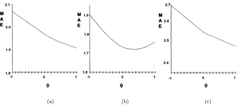
From the plots in Fig. 12 the optimal choice of ˆ

fφ(x) is always between the hybrid model,φ= 0, and the bootstrap predictor, φ= 1. For the bulk of the out of sample data, the best choice of φis between 0.3 or 0.4. However for the first month after the training set in Fig. 12(a), the bootstrap predictor,

φ= 1, does the best. This is partially because of the slow degradation of the network, as the training set becomes more distant. It is also due to expiry dates. During the five-month period in Fig. 12(b), a set of options expires. During periods of expiry and low volatility, the option price is fairly well determined and this is reflected by the lower mean absolute error for this period.

s_{It was not necessary to adjust the cash-flows when calculating the sharpe ratio as it was assumed that most options expired on the}

same day and the premium is paid upon option expiry.

t_{The relationship between bagging and bootstrap was not made explicit by (Breiman, 1994). (Efron and Tibshirani, 1993), p. 125}

(a) (b) (c)

Fig. 12. The mean absolute error of ˆfφ(x) is shown as a function ofφ. (a) First month (b) Next 5 months (c) Deep out

of the money. The average out of sample performance suggests that a model between the “hybrid” predictor and the bootstrap predictor is best. At the edges of the input space, shown in plot (c) the bootstrap predictor is best.

0.02 0.07

0.13 0.19

0.25 0.31

-0.001 -0.0005 0 0.0005 0.001 0.0015

ERROR (C/X)

F/X

T-t

0.

96

0.

87 0. 90 0.₉₃ 0.

99 1.02 1.05

Fig. 13. The bagging hybrid surface when standard

de-viationσ= 0.11.

Deep-inorout-of-the-moneypricing is not impor-tant when options expire, but is very imporimpor-tant at other times. Deep-in or out-of-the-money options are also interesting because they exist at the edge of the input space in the training set. No technique is good in providing accurate estimates at the edge of the training set. The neural networks sigmoid func-tions usually level out and under/over shoot posi-tive/negative trends. This behavior is even worse in bagging predictors derived from the original hy-brid network. The bootstrap assumption works very well at the edge of the data set as exemplified by Fig. 12(c). The bootstrap predictor does best in this region.

0.02 0.07

0.13 0.19

0.25 0.31

-0.001 -0.0005 0 0.0005 0.001 0.0015 0.002

ERROR (C/X)

F/X

T-t

0.96

0.87 0.90 0.93

0.99 1.02 1.05

Fig. 14. The bagging hybrid surface when standard

de-viationσ= 0.2.

The best choice for φ will vary over the input space of the predictor,out-of-the-moneyoptions are more biased than other options. In addition, model fits at the edge of the data set, as demonstrated by the deep out of the money options, appear to suffer from the most bias; in these areas the bootstrap pre-dictor, φ = 1, is very good. The steady decline as

φ goes from 0 to −1 reflects badly on the bagging predictor.

0.9

6

0.8

7

0.9

0

0.9

3 0.9₉ 1.0

2

1.0

5

0.02 0.07

0.13 0.19

0.25 0.31

-0.001 -0.0005 0 0.0005 0.001 0.0015 0.002

ERROR (C/X)

F/X

T-t

Fig. 15. The bagging hybrid surface when standard

de-viationσ= 0.28.

samples. In addition, the function we are learning is nonlinear but very smooth. Our results suggest that for an well-approximated function, bootstrap bias re-duction methods are preferable to bagging.

It is interesting to make comparisons between the hybrid pricing surfaces (Figs. 3–5) and the bagging pricing surfaces (Figs. 13–15). The surfaces are very similar, however there are some subtle differences. The main difference is that the bagging hybrid sur-faces are shifted up — the errors are almost all above zero. This is very interesting and quite unexpected.

6. Estimation of Bias Using Bootstrap Techniques

The large majority of option pricing research involves finding a model that fits the data. Very little research has been done on generating bias estimates for new models. The bias of an estima-tor θ is the difference between the expected value of the estimator and the true value of the parame-ter Bias(θ) =θ−E(θ). Ifθ is the hybrid ANN the Bias(Hybrid ANN) = fhybrid −fbag from Eq. (5). The bias estimate is useful because it can show the regions of input space in which the bias becomes se-rious. In these regions, the estimator is poor and an alternative estimator may be considered.

The bootstrap estimate of bias for a hybrid neu-ral network as a function ofF/X,time to maturity, and a low implied volatility is shown in Fig. 16. For this particular implied volatility, the neural network is showing a large bias for in the money options that are near maturity. In this region, there is a rela-tively sparse amount of training data because op-tions are typically written out-of-the-money. This region is also at the edge of the training set because

0.87

0.96

1.05 0.02

0.07 0.13 0.19 0.25 0.31

0 0.0002 0.0004 0.0006 0.0008 0.001

0.0012

BIAS

F/X T-t

Fig. 16. Estimate of the bias using bootstrap techniques

at standard deviationσ= 0.11.

of its nearness to expiry and is showing some of the poor generalization that often occurs at the edge of the data with nonparametric regression techniques. This observation motivates further work which shall utilize the inherent option pricing model boundary conditions and utilize a novel ANN architecture so to constrain the ANN at the option pricing bound-ary conditions (Lajbcygier, 1998).

7. Summary

A hybrid neural network was created to predict the difference between conventional parametric models and observed option prices. Bootstrap methods al-lowed trading strategies to be developed which avoid spurious trades due to incorrect model fits. Mod-ified bootstrap predictors based on a weakening of the bootstrap assumption for bias was used to com-pare bagging, hybrid and bootstrap predictors. It was concluded that somewhere between the hybrid and the bootstrap predictor is best for this option-pricing problem. Bootstrap methods for bias reduc-tion was shown to give good results at the edge of input space where good extrapolation is critical.

Acknowledgements

References

Y. Ait-Sahalia and A. Lo 1995, “Nonparametric estima-tion of state-price densities implicit in financial asset prices,” working paper, MIT-Sloan School.

C. Ball and A. Roma 1994, “Stochastic volatility option

pricing,”J. Financial Quant. Anal.29(4), 589–607.

D. Bates 1997a, “The skewness premium: Option

pric-ing under asymmetric processes,” Adv. Futures and

Options Res.9, 51–82.

D. Bates 1997b, “Post -’87 crash fears in S&P 500 futures options,” working paper, Department of Finance, University of Iowa.

W. Baxt and H. White 1995, “Bootstrapping confidence intervals for clinical input variable effects in a network trained to identify the presence of acute myocardial infraction,” Neural Comput.7, 624-638.

C. Bishop 1995, Neural Networks For Pattern

Recogni-tion(Clarendon Press).

F. Black and M. Scholes 1973, “The pricing of options and corporate liabilities,”J. Polit. Econ.81, 637–654. L. Breiman 1994, “Bagging predictors,” Technical Re-port No. 421, Department of Statistics, University of California at Berkeley.

M. Brenner and D. Galai 1981, “The properties of the estimated risk of common stocks implied by op-tion prices,” Working Paper No. 112, University of California at Berkeley.

L. Canina and S. Figlewski 1993, “The informational con-tent of implied volatility,”Rev. Financial Stud.6(3), 659–668.

D. Chiras and S. Manaster 1978, “The informational con-tent of option prices and a test of market efficiency,”

J. Financial Econ.6, 213–234.

B. Christensen and N. R. Prabhala 1994, “On the dy-namics and information content of implied volatility: A bivariate time series perspective,” working paper, Stern School of Business.

G. Chryssolouris, M. Lee and A. Ramsey 1996, “Confi-dence interval prediction for neural network models,”

IEEE Trans. Neural Networks7(1), 229–232. C. J. Corrado and J. T. W. Miller 1996a, “Efficient

option-implied estimators,”J. Futures Markets16(3),

247–272.

T. Day and C. Lewis 1992, “Information content of im-plied volatilities,”J. Econometrics52, 267–288.

E. Derman and I. Kani 1994, “Riding on a smile,”Risk

7(2), 32–39.

E. Derman, I. Kani and J. Zou 1996, “The local volatil-ity surface: Unlocking the information in index option

prices,”Financial Anal. J.July/August, 25–36.

F. Diz and T. Finucane 1993, “The time series proper-ties of implied volatility of S&P 100 index options,”

J. Financial Eng.2(2), 127–154.

B. Dumas, J. Fleming and R. Whaley 1996, “Implied volatility functions: Empirical tests,” working paper, Centre for Research on Economic and Policy Reform (CEPR) research programme, Stanford University.

J. Eales and R. Hauser 1990, “Analysing biases in

valua-tion models of opvalua-tions on futures,”J. Futures Markets

10(3), 211–228.

B. Efron and R. J. Tibshirani 1993, An Introduction to

the Bootstrap(Chapman and Hall, New York). R. Engle and C. Mustafa 1992, “Implied ARCH models

from options prices,”J. Econometrics 52, 289–311.

S. Figlewski 1997, “Forecasting volatility,” Financial

Markets,Institutions & Instruments6(1), 1–88. J. Fleming, B. Ostediek and R. Whaley 1995, “Predicting

stock market volatility: A new measure,” J. Futures

Markets15(3), 265–302.

R. Geske and K. Kim 1994, “Regression tests of volatil-ity forecasts using Eurodollar futures and options contracts,” working paper No. 31–93, University of California at Los Angeles.

T. Gilmore 1997, Correspondence with BZW futures broker — T. Gilmore, Melbourne, Australia. N. Gultekin, R. Rogalski and S. Tinic 1982, “Option

pric-ing model estimates, some empirical results,”

Finan-cial ManagementSpring 1982, 58–69.

D. Guo 1996, “The predictive power of implied stochastic

variance from currency options,”J. Futures Markets

16(8), 915–942.

J. A. Hammer 1989, “On biases reported in studies of the

Black-Scholes option pricing model,”J. Econ.

Busi-ness41, 153–169.

R. Heynen 1994, “An empirical investigation of observed smile patterns,” working paper, Tinbergen Institute, Erasmus University, Rotterdam, Netherlands. J. Hull and A. White 1987, “The pricing of options on

assets with stochastic volatility,”J. FinanceXLII(2), 281–300.

J. Hutchinson, A. Lo and T. Poggio 1994, “A non-parametric approach to pricing and hedging

deriva-tive securities via learning networks,”J. Finance

XLIX(3), 851–890.

E. Jacquier and R. Jarrow 1996, “Model error in contin-gent claim models,” working paper, Johnson Gradu-ate school of Management, Cornell University. B. Jacquillant, J. Hamon, P. Handa and R. Schwartz

1993, “The profitability of limit order on the paris

stock exchange,” working paper, Universit´e Paris

Dauphine.

R. Jarrow and J. Wiggins 1989, “Option pricing and im-plicit volatilities,”J. Econ. Surveys3, 59–80. H. Johnson and D. Shanno 1987, “Option pricing when

the variance is changing,”J. Financial Quant. Anal.

22(2), 143–151.

P. Jorion 1995, “Predicting volatility in foreign exchange

market,”J. FinanceL(2), 507–528.

P. Lajbcygier 1998, “Improving option pricing using neu-ral networks and bootstrap methods,” PhD thesis, School of Business Systems, Monash University. P. Lajbcygier, C. Boek, M. Palaniswami and A.

Flitman 1995, “Neural network pricing of all

ordinar-ies options on futures,”Proc. Third Int. Conf.

eds. A-P. Refenes, Y. Abu-Mostafa, J. Moody and A. Weigend (World Scientific, Singapore), pp. 64–77. P. Lajbcygier and J. Connor 1997, “Improving option

pricing with bootstrap,” Int. Conf. Neural Networks

(IEEE Press: New York).

P. Lajbcygier and A. Flitman 1996, “A compar-ison of non-parametric regression techniques for the pricing of options using an implied volatility,”

Decision Technologies for Financial Engineering:

Proc. Fourth Int. Conf. Neural Networks in the Cap-ital Markets (NNCM’96) eds. A. S. Weigend, Y. S. Abu-Mostafa and A.-P. Refenes (World Scientific, Singapore), pp. 201–213.

C. G. Lamoureux and W. D. Lastrapes 1993, “Forecast-ing stock-return variance: Towards an understand-ing of stochastic implied volatilities,” Rev. Financial Stud.6(2), 283–326.

H. Latane and R. Rendleman 1976, “Standard devia-tions of stock price ratios implied in option prices,”J. Finance31(2), 369–381.

B. Le Baron and A. S. Weigend 1998, “A Bootstrap eval-uation of the effect of data splitting on financial time

series”,IEEE Trans. Neural Networks9(1), 213–220.

C. Martini and S. Taylor 1995, “Test of the modifed Black formula for options on futures,” working paper, Department of Accounting & Finance, Melbourne University.

S. Mayhew 1995, “Implied volatility,”Financial Anal. J.

July–August,8(18), 8–19.

R. C. Merton 1973, “Theory of rational option pricing,”

Bell J. Econ. Management Sci.4, 141–183.

M. Ncube 1996, “Modeling implied volatility with OLS

panel data models,” J. Banking and Finance 20,

71–84.

H. Park and R. Sears 1985, “Estimating stock index fu-tures standard deviation through the price of their

options,”J. Futures Markets5, 223–237.

G. Pass 1993, “Assessing and improving neural

net-work predictions by the Bootstrap algorithm,”

Ad-vances in Neural Information Processing5, eds. S. J. Hanson, J. D. Cowan and C. L. Giles (Morgan Kaufman), pp. 196–203.

S. Phillips and C. Smith 1980, “Trading costs for listed

options: The implications for market efficiency,” J.

Financial Econ.179–120.

A.-P. N. Refenes and F. G. Miranda 1996, “A principled approach to neural model identification and its ap-plication to intraday volatility forecasting,” working paper, London Business School.

B. Resnick, A. Sheikh and Y. Song 1993, “Time varying volatilities and the calculation of the weighted

im-plied standard deviation,”J. Financial Quant. Anal.

28(3), 417–430.

R. Roll 1984, “A simple implicit measure of the

ef-fective bid-ask spread in an efficient market,” J.

Finance39, 1127–1140.

M. Rubinstein 1985, “Nonparametric tests of alterna-tive option pricing models using all reported trades and quotes on the 30 most active cboe option classes

from August 23, 1976 through August 31, 1978,” J.

FinanceXL(2), 455–480.

M. Rubinstein 1994, “Implied binomial trees,”J. Finance

49(2), 771–818.

K. Shastri and K. Tandon 1986, “An empirical test of a valuation model for American options on futures

con-tracts,”J. Financial Quant. Anal.21(4), 377–392.

R. Tibshirani 1996, “A comparison of some error

esti-mates for neural network models,” Neural Comput.

8, 152–163.

C. Turvey 1990, “Alternative estimates of weighted im-plied volatilities from soybean and live cattle

op-tions,”J. Futures Market10(4), 353–366.

X. Xu and S. Taylor 1995, “Conditional volatility and the information efficiency of the PHLX currency options