A COMPARISON OF MARGIN CALCULATION METHODS FOR CONTRACTS ON EXCHANGE TRADED SECURITIES

Mathematical statistics

A COMPARISON OF MARGIN CALCULATION METHODS

FOR CONTRACTS ON EXCHANGE TRADED SECURITIES

by

Mattias Bylund

Department of Mathematics

Royal Institute of Technology

FOR CONTRACTS ON EXCHANGE TRADED SECURITIES

The main objective of this thesis is to analyse methods used by clearing organisations for calculating

margin requirements on contract portfolios. Margin requirements are calculated to protect the

clearinghouse in case of an unfavourable market outcome. Methods analysed include SPAN, TIMS

and OMS II, these are compared with each other theoretically and with the help of simulations. The

comparisons are not made to rank the methods but rather to highlight differences between them.

Summary in Swedish

När två parter går in i ett terminskontrakt så tar de på sig skyldigheten att köpa respektive sälja den

underliggande varan till det specificerade priset på slutdagen. I fallet med en option så är det

utfärdaren som har skyldigheten att köpa respektive sälja den underliggande varan på slutdagen.

Detta gör att båda parter har en risk i kontraktet, nämligen risken att motparten inte kan fullfölja sina

åtaganden på slutdagen. För att komma runt denna risk så går ett clearinghus in som motpart i alla

sådana kontrakt, dvs clearinghuset garanterar att alla kontrakt blir utförda. Clearinghuset tar ut ett

säkerhetskrav av alla som har en skyldighet i ett kontrakt, detta för att clearinghuset skall kunna

skydda sig självt mot möjliga framtida förluster.

I would like to thank my supervisor Erik Aurell, at the Department of Numerical Analysis and

Computer Science at the Royal Institute of Technology, for his help with mathematical issues in this

thesis.

1

I

NTRODUCTION

...7

2

M

ARGINMETHODS

...8

2.1 Standard Portfolio Analysis of Risk...8

2.2 Theoretical Intermarket Margining System...11

2.3 OM “Window Method”...13

3

P

ORTFOLIOANDCONTRACTVALUATION

...16

3.1 Formulas used when pricing options...16

3.1.1 Black & Scholes...16

3.1.2 Black 76...18

3.1.3 Binomial model for American put...20

3.2 Calculating “risk margin” in each scan point...22

3.2.1 Margining contracts in OMS II...22

3.2.2 Margining contracts in SPAN...24

3.2.3 Margining contracts in TIMS...25

3.2.4 Comparison...25

3.3 Taking correlation into account...26

3.3.1 The Window method...26

3.3.2 TIMS...27

3.3.3 SPAN...28

3.3.4 Comparison...31

4

E

STIMATINGPARAMETERS

...32

4.1 Estimating a valuation interval...32

4.2 Estimating windows between different underlying securities...36

4.4 SPAN Specific Parameters...37

4.4.1 Inter-Month Spread Charge...37

4.4.2 Short Option Min. Charge...37

4.4.3 Inter-Commodity Concession...37

4.4.4 Delta Spread Ratios...37

4.5 TIMS Specific Parameters...37

5.4.1 Futures Spread Margin...37

5.4.2 Options Spread Margin...37

5

S

IMULATIONS

...38

5.1 Simulating risk margin...38

5.1.1 Futures...38

5.1.2 Options...39

5.2 Portfolios with inter month margin...40

5.2.1 Futures...40

5.2.2 Options...43

5.3 Portfolios with contracts on different underlying...46

5.3.1 Futures...47

5.3.2 Options...49

6

C

ONCLUSIONS

...54

7

S

UGGESTIONSFORFURTHERINVESTIGATIONS

...56

A

PPENDIX

A...57

Glossary...57

A

PPENDIX

B...58

Delivery Margin...58

A

PPENDIX

C...60

Visual Basic Scripts...60

1

Introduction

When an option trade is made between a buyer and a seller the buyer receives the

right

to

buy or sell the underlying commodity at the strike price at a given time in the future. On the

other hand the seller of the option has made an

obligation

to buy or sell the underlying

commodity at the strike price at a given time in future.

In the case of a forward or future both the buyer and the seller have made an obligation to

buy or sell the underlying commodity at a predetermined price at a given time in the future.

In the option case the buyer faces a risk that the seller fails to fulfil his obligation in case of

an unfavourable change in the price of the underlying commodity. In the case of a forward

or a future both parties faces this risk. Such possible failures give rise to questions about the

credit worthiness of the counterparty.

This problem is solved by the existence of a clearinghouse. One of the main functions of

the clearinghouse is to guarantee that all contracts traded are honoured. The clearinghouse

serves as counterparty in all transactions, that is, the clearinghouse becomes the buyer to

every seller, and the seller to every buyer.

Acting as counterparty, and guaranteeing all transactions, the clearinghouse eliminates any

questions about credit worthiness of the original counterparty. This also permits a

secondary market for the contract to work more efficiently, since a market participant can

close a position without recourse to the original counterparty.

However, the clearinghouse will now face the risk that a member or a client may fail to

fulfil his obligation in case of an unfavourable change in the price of the underlying

commodity. In case of a member failing to fulfil his obligation the clearinghouse is obliged

to neutralise the position of the failing member.

To protect the clearinghouse in such cases each participant with an obligation has to pledge

collateral. The collateral could be cash, stocks, bonds or other financial instruments. The

amounts of collateral to be pledged is called

margin requirement

.

Important demands on the margin requirement are:



Not too small, since the clearinghouse may then loose money



Not too high, since this may discourage trading.

To determine the margin requirement one uses a margin calculation algorithm. There are

several algorithms in use by clearinghouses around the globe. Three of these margin

calculation procedures are to be analysed in this thesis. These are the most common one,

Standard Portfolio Analysis of Risk

(SPAN), developed by the Chicago Mercantile

Exchange (CME), the

Theoretical Intermarket Margining System

(TIMS), developed by

the Options Clearing Corporation (OCC), and the

“Window Method”,

developed by OM

2

Margin methods

The ideas of the three algorithms are basically the same. The cost to neutralise an account

immediately is the account’s negative market value. If it were possible to close an account

in the same time as a member fails to pledge collateral, this negative market value would

equal the margin requirement. This is normally not the case, and during the time it takes to

neutralise an account, a negative value can increase in a rapidly falling/rising market. This

calls for a simulation of the maximal neutralisation cost during a specified time frame. To

do these simulations a valuation interval for all option and future series based on historical

fluctuations of the underlying instrument is constructed. The valuation interval specifies

how much the clearinghouse believes the price of the underlying can change during a one

to two days time horizon. Additionally, for option contracts the clearinghouse has to take

into consideration possible changes in volatility over the one to two days time. For

portfolios containing several instruments one has to take into account the possibility of

different price correlation when one adds the margin requirements for each instrument.

To calculate the cost of closing an option position, different pricing formulas are used.

These are specified by the clearinghouse using the margining procedure and not by the

margining procedure itself. The models used by “Stockholmsbörsen” are:



Black & Scholes



Black-76



Binomial model

A further explanation of the pricing formulas and their usage will be presented later on

in the beginning of chapter 3.

2.1 Standard Portfolio Analysis of Risk

The Standard Portfolio Analysis of Risk, or SPAN, method is a margining system

developed by the Chicago Mercantile Exchange (CME) in 1988. In brief, SPAN calculates

worst case loss scenarios on a contract portfolio, adjusting this loss for net premium cost or

benefit from liquidating any option position, and finally adjusting for any offsetting profits

generated by closely correlated portfolios in other contracts.

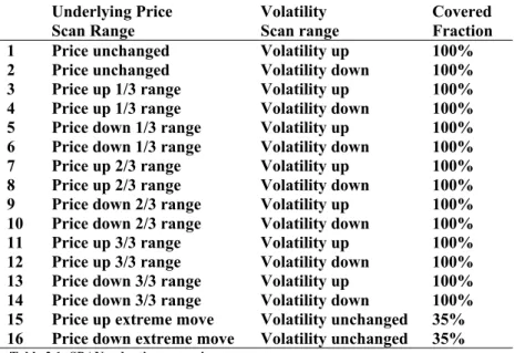
In SPAN the valuation interval is divided into 8 possible up or down moves, additionally

for each up or down move the volatility can either increase or decrease. This gives us 16

alternative market scenarios to calculate the profit or loss a portfolio will make.

Underlying Price

Scan Range

Volatility

Scan range

Covered

Fraction

1

Price unchanged

Volatility up

100%

2

Price unchanged

Volatility down

100%

3

Price up 1/3 range

Volatility up

100%

4

Price up 1/3 range

Volatility down

100%

5

Price down 1/3 range

Volatility up

100%

6

Price down 1/3 range

Volatility down

100%

7

Price up 2/3 range

Volatility up

100%

8

Price up 2/3 range

Volatility down

100%

9

Price down 2/3 range

Volatility up

100%

10

Price down 2/3 range

Volatility down

100%

11

Price up 3/3 range

Volatility up

100%

12

Price up 3/3 range

Volatility down

100%

13

Price down 3/3 range

Volatility up

100%

14

Price down 3/3 range

Volatility down

100%

15

Price up extreme move

Volatility unchanged

35%

16

Price down extreme move

Volatility unchanged

35%

Table 2.1: SPAN valuation scenarios

Mathematically one can view the risk calculations performed in SPAN as producing the

maximum of the expected loss under each of sixteen probability measures. For the first

fourteen scenarios the probability measures are point masses at each of the fourteen points

in a space



of securities prices and volatilities. The case of extreme moves corresponds to

taking the convex combination (0.35, 0.65) of the losses at the extreme move point under

study and the no move at all point.

The largest loss across these 16 scenarios is the “scanning risk” for the contract. For a

portfolio consisting of contracts valued together, the “scanning risk” equals the largest loss

given each scenario, added together for each contract. To achieve the total margin

requirement this figure is adjusted for inter-month margins, inter-commodity concessions

and spot month isolation. These adjustments are done because in calculating the scanning

risk one does not take in to account the inter-month spread movements and one assumes

perfect correlation between delivery months. The total margin calculation can be written as:

Total Initial Margin = Scanning Risk + Inter-Month Risk – Inter Commodity Spread

– Net Option Value

1

A description of the ingoing entities follows:

The Net Option Value is only used for equity options also called security style options. The

Net Option Value reflects the current market value of the option position(s). Liquidating a

long option position will generate a cash equivalent to the current premium, while

liquidating a short option position will have a cost equal to the current premium. For a

portfolio containing only long positions the Net Option Value will always be at least

equivalent to the scanning risk, so no initial margin collateral is required.

1

_{Note: All three margin methods (SPAN, TIMS and OMS) also handles the risk}

Before we continue with the two last entities let’s look at the scanning risk yet again. The

16 valuation points are used to create a risk array. This risk array is calculated by the

clearinghouse. One risk array is calculated for each traded contract at all exchanges cleared

by the clearinghouse. In calculating the risk arrays one takes the difference between the

original option value (settlement value) and the recalculated option value, given the

relevant scenario. The margin for a portfolio of contracts is then determined by multiplying

each array value by the contract size. This gives the scanning risk for each contract. The

largest loss is determined by adding each scan point value for a contract to the other

contracts corresponding scan point value, i.e.

scanpoint1(contract1)+scanpoint2(contract2)

+ scanpoint3(contract3)+…

and then taking the maximum value of the 16 values achieved.

In SPAN methodology the maximum loss is represented by the largest positive value.

Now, these risk arrays are delivered in a Risk Parameter File together with composite delta.

Delta values measure the rate of change of the price of a derivative with the price of the

underlying asset. The delta of a derivative with price

f

is

Δ

=

∂

f

∂

S

_{. Future deltas are}

always 1.0 whereas options deltas range from –1.0 to +1.0 (0 to +1.0 for long calls and 0 to

–1.0 for long puts, the opposite holds for short calls and puts). The option deltas are

dynamic, i.e. a change in value of the underlying will not only affect the options price but

also its delta statistics. The composite deltas are delivered as a probability weighted

average of a set of delta values, each of which is calculated under the 16 scenarios above.

One can view the composite delta for an options contract as the best estimate of what the

contract’s delta will be after the lookahead time has passed. These composite deltas are

used in SPAN during the calculation of month spread charges and for

inter-commodity credits.

The inter-month risk charge, is used because of the potential for a less than perfect

correlation between different delivery dates; i.e. the inter-month risk margin covers the

calendar basis risk that may exist for portfolios containing futures and options with

different expirations. SPAN identifies the net delta associated for each futures contract or

other underlying instrument in which the portfolio has positions. The spreads are then

formed using these net deltas according to patterns specified in the SPAN risk parameter

file. When spreads are formed, SPAN keeps track, for each tier, which is a set of

consecutive future contracts, of how much delta has been consumed by spreading for the

tier, and how much remains. Then for each spread formed, a charge is assessed per spread

at the specified charge rate for the spread. The inter-month spread charge is then the total of

all these charges for a particular combined commodity.

Inter-commodity spread is used to recognise the risk reducing aspects of portfolios

containing positions in related instruments. This is so because price movements tend to

correlate fairly well between related underlying instruments. Often, as prices of related

instruments move, they tend to do so in tandem. It is not probable that one instrument

increases in price and another closely related instrument decreases in price at the same

time. This leads to the conclusion that gains from held/written positions in one instrument

may sometimes offset losses from written/held positions in another related instrument.

SPAN identifies the net delta for each contract month, and for the underlying instrument as

a whole, and then processes the inter-commodity spread data

2

_{contained in the risk}

parameter file to form spreads between the combined commodities. The spreads are formed

with the use of the deltas a more thorough explanation of this is contained in section 3.3.3.

For some portfolios it will be possible to form a multitude of inter-commodity spreads.

Highest priority is often given to those spreads that generate the largest monetary value

savings and the lowest priority to those that generate the smallest savings. That is, with

reference to historical data one sets the order of the spreads so that the ones generating the

highest savings comes first in the table and those that generates the lowest savings comes

last. If the order of the spreads were not set in the described way the delta could be

consumed before the largest offset could be applied. According to what is stated below this

would lead to a higher margin requirement. Now each spread generates a percentual saving

from the outright margin requirement for the underlying instruments involved. The

percentages are applied to these outright requirements and in most cases this results in a

lower net requirement for the instrument (the case of no lowered net requirement of course

means that the net requirement is the same).

As the total initial margin is calculated SPAN sets the final margin requirement according

to the following procedure. The total initial margin (excluding any Net Option Value that

may exist) is compared with the Short Option Minimum charge, and then the margin

requirement is set to the largest value of these two.

The Short Option Minimum charge is set because of short option positions in extremely

deep-out-of-the-money strikes may seem to have little or no risk across the entire scanning

range. But if the underlying market condition change sufficiently these options may move

into-the-money and generate large loss for the holders of short positions in these options.

One can therefore describe SPAN as the following maximum:

SPAN

_Risk

=

max

(

Risk margin

+

inter-month margin

+

inter-commodity spread,

Short Option Minimum Margin

)+

Net Option Value

2.2 Theoretical Intermarket Margining System

3

The Theoretical Intermarket Margining System or TIMS method was originally developed

1986 in Chicago by the Options Clearing Corporation (OCC). This is used to calculate

margin requirements on its options and futures contracts, comprising a daily mark to

market margin (or premium margin that equals the Net Option Value in SPAN) plus a

cushion to cover the risk of an adverse price change (risk margin). It also contains a futures

spread margin. TIMS organises all classes of options and futures relating to the same

underlying asset into class groups and all class groups whose underlying assets exhibit

close price correlation into product groups.

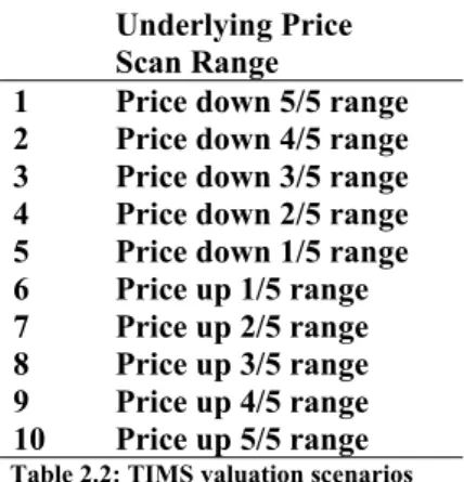
In TIMS methodology the valuation interval is divided into ten different valuation points.

These consist of five downside values and five upside values. No consideration is taken to

the possibility of a change in volatility.

3

_{Note: TIMS is here described as it is in [6], there may be differences in this}

method from the original one developed by the OCC in Chicago. Due to

Underlying Price

Scan Range

1

Price down 5/5 range

2

Price down 4/5 range

3

Price down 3/5 range

4

Price down 2/5 range

5

Price down 1/5 range

6

Price up 1/5 range

7

Price up 2/5 range

8

Price up 3/5 range

9

Price up 4/5 range

10

Price up 5/5 range

Table 2.2: TIMS valuation scenarios

Equivalently to SPAN the TIMS calculations can be viewed as producing the maximum of

the expected loss under each of ten probability measures. For all ten scenarios the

probability measures are point masses at each of the ten points in the space



of securities

prices.

Each scenario is subtracted with the settlement value for the contract. The largest loss

across these ten scenarios is the risk margin for the contract. For a portfolio containing

different contracts on different underlyings TIMS adds up the values for each class group

exactly as SPAN adds its values. If the class group is not part of a bigger product group the

maximum loss is taken as the risk margin for the class group. However if the class group is

part of a bigger product group and we have offsetting values only a percentage of these

(around 30%) are added to the other class group values. Again the largest loss is taken as

the product group margin. To provide additional protection in the calculation of risk

margin, the value of deep out-of-the-money short call positions at the maximum upside and

deep out-of-the-money short put positions at the maximum downside is presumed to be at

least a fixed percentage of the margin interval.

The total margin calculation in TIMS consists of:

Total Margin = Futures Spread Margin + Risk Margin + Premium Margin

The futures spread margin covers futures positions, which have been spread between

different expiry months. TIMS applies a charge to these spreads to cover any risk involved

in these spreads.

price. The premium margin is as in SPAN methodology only calculated for securities style

options. For a portfolio consisting of several option contracts the premium margin for each

class group is calculated by subtracting the market value of the long positions from the

market value of the short positions.

If the risk margin for a particular product group is less than a calculated minimum margin,

that is similar to the short option minimum charge in SPAN, for this product group, then

this minimum margin is taken as the risk margin. TIMS only compares this minimum

margin to the risk margin and not to the total margin.

For a multiple security portfolio the risk and premium margin is calculated in four steps:

1. Calculate separate portfolios

2. Calculate total premium margin

3. Calculate total risk margin

4. Apply offsets to risk margins

2.3 OM “Window Method”

OMS II or the “Window method” or the “Vector method” is the OM risk calculation

method for calculating margin requirements. It is included in the risk valuation or RIVA

system within OM SECUR. It was constructed in order to handle non-linear instruments in

a better way than SPAN or TIMS. OMS II calculates worst case loss scenarios, store these

in vectors, adjust for spreading, and adds the vector in a way that takes correlation in to

account. This will be described later on in this chapter.

In OMS II the valuation interval is divided into n (normally n=31) possible up or down

moves, additionally for each up or down move the volatility can either increase stand still

or decrease. This gives us 93 alternative market scenarios (if n=31) to calculate the profit or

loss a portfolio will make.

The scenario with no price move at all is the middle scenario and around it there are 15 up

and 15 down scenarios (or

(n-1)/2

up and

(n-1)/2

down scenarios).

Underlying Price

Scan Range

Volatility

Scan range

1

Price unchanged

Volatility down

2

Price unchanged

Volatility unchanged

3

Price unchanged

Volatility up

4

Price up 1/15 range

Volatility down

5

Price up 1/15 range

Volatility unchanged

6

Price up 1/15 range

Volatility up

7

Price down 1/15 range

Volatility down

8

Price down 1/15 range

Volatility unchanged

9

Price down 1/15 range

Volatility up

10

Price up 2/15 range

Volatility down

11

Price up 2/15 range

Volatility unchanged

12

Price up 2/15 range

Volatility up

.

.

.

.

.

.

.

.

.

88

Price up 15/15 range

Volatility down

89

Price up 15/15 range

Volatility unchanged

90

Price up 15/15 range

Volatility up

91

Price down 15/15 range

Volatility down

92

Price down 15/15 range

Volatility unchanged

93

Price down 15/15 range

Volatility up

Table 2.3: OMS valuation scenarios. (n=31)

Yet again, as in both SPAN and TIMS, one can view OMS II mathematically as producing

the maximum of the expected loss under each of 93 probability measures. For all 93

scenarios the probability measures are point masses at each of the 93 points in a space



of

securities prices and volatilities.

Each valuation point is saved in a 3x31 matrix, that is, each row contains a price move and

the three volatility fluctuations. The matrix is expanded to a 6x31 matrix so that the case of

both a bought and sold contract is represented in the matrix, this because of additional

fine-tunings that are available in OMS II. These matrixes are saved for use when margin

requirements of portfolios are calculated.

In the case of an account containing positions of two or more types of contracts the risk of

the position is the combined risk characteristics of the different contracts registered to the

account. To take the offsetting characteristics of the instrument into account one talks about

cross margining. The default cross margining divides the positions into one group per

underlying. Positions on instruments within the same underlying are said to be totally

correlated. The default cross margin can be described as instruments with the same

underlying being totally correlated and instruments with different underlying being

uncorrelated. During a default cross margin run a portfolio with instruments on the same

underlying will add the valuation files pointwise as in SPAN and then take the largest

negative value as the margin requirement for the portfolio

4

_{. If the portfolio consists of}

instruments on different underlyings the largest negative value of each valuation file will be

added.

However, a method such as default cross margining does not take correlations between

different underlyings or different expiry months into consideration. Therefore in OMS II

one uses the so-called “Window method” when a portfolio containing instruments on

different underlyings or contracts with different expiry months is margined.

In the window method, the different instruments are sorted into a number of groups, called

window classes. The window classes have a window size defined in percent. When the

percentage goes down the correlation goes up and vice versa, e.g. a window size of 0%

means that the instruments in the window class are totally correlated and a window size of

100% means that the instruments in the window class are uncorrelated. There is also a

possibility for a window class to be a member of another window class, and in such case

creating a tree structure of more complicated correlations. To calculate the margin for a

4

_{Note: In OMS II the margin requirement is represented as the largest negative}

3

Portfolio and contract valuation

3.1 Formulas used when pricing options

The use of option pricing formulas when valuing an option contract during the calculation

of margin for a portfolio depends heavily on which clearinghouse that is using the

margining algorithm. Since this thesis is performed at OM, the methods described for

valuing different options are the ones that are in use by OM, other clearing organisations

may use different pricing formulas. As an example, the Options Clearing Corporation, that

has developed the TIMS method, uses the Cox-Ross-Rubinstein binomial model for

valuing all its contracts.

Product Without dividend With dividend

Yield With discrete Dividend American call based

on spot Black & Scholes Binomial Binomial withDividends American put based

on spot Binomial if interest rate is non-zero Black & Scholes if interest rate is zero

Binomial Binomial with

Dividends

American opt on real

Future Binomial if interest rate is non-zero Black & Scholes if interest rate is zero

Binomial using r-q when calculating probabilities, And r when discounting backwards in the tree

Binomial with Interest rate r

European opt based

on spot Black & Scholes Black & Scholes modified By also using q

Discount spot with dividends, then use Black & Scholes European opt based

on future Black – 76 Black – 76 (no q) Black –76

Table 3.1: Option valuation formulas, (for description se appendix)

3.1.1 Black & Scholes

The Black & Scholes model is used to set theoretical prices on European put and call

options.

In the Black & Scholes model one assumes two securities: B the price process of a risk free

asset and S the price process of a stock. These processes are assumed to follow a system of

stochastic differential equations:

{

dB

(

t

)=

rB

(

t

)

dt

¿ ¿¿¿

Where

r , μ , σ

are real constants.

Now suppose that

f

(

t

)=

F

(

t , S

t

)

_{is the price of some derivative contingent on}

_S

_{at time}

t

. Let us construct a self financing portfolio

I

consisting of the stock

S

and the derivative

f

dI

=

α df

+

β dS

=

{

Itô

}

=

=

α

(

(

f

_t

+

μ Sf

_S

+

1

2

σ

2

_S

2

_f

SS

)

dt

+

σ Sf

S

dW

)

+

β

(

μ Sdt

+

σ SdW

)

=

α

(

f

_t

+

μ Sf

_S

+

1

2

σ

2

_S

2

_f

SS

)

dt

+

βμ Sdt

+

(

αf

S

+

β

)

σ SdW

Now assuming that the portfolio

I

is riskless; i.e.

β

=−

αf

S

_{, so that}

dI

=

α

(

f

_t

+

μSf

_S

+

1

2

σ

2

_S

2

_f

SS

)

dt

+

βμ Sdt

=

α

(

f

_t

+

μSf

_S

−

μ Sf

_S

+

1

2

σ

2

_S

2

_f

SS

)

dt

=

α

(

f

_t

+

1

2

σ

2

_S

2

_f

SS

)

dt

If we further assume that the existence of an arbitrage opportunity is precluded, i.e.

dI

=

rIdt

_{, we obtain}

dI

=

r

(

αf

+

βS

)

dt

=

r

₍

αf

−

α Sf

_S

₎

dt

We obtain

f

_t

+

rSf

_S

+

1

2

σ

2

_S

2

f

SS

=

rf , t

<

T

f

(

t

)

=

F

(

S ,T

)

This is the Black & Scholes differential equation. Solving this equation with

f

_t

=max

(

S

(

T

)−

X ,

0

)

_{for a European call or}

f

t

=max

(

X

−

S

(

T

)

,

0

)

_{for a European}

put option yields the Black & Scholes formulas for the prices at time zero.

The Black & Scholes prices of a European call option on a non-dividend-paying stock and

a European put option on a non-dividend-paying stock are:

c

=

S

₀

N

₍

d

₁

₎

−

Xe

−rT

N

₍

d

₂

₎

and

p

=

Xe

−rT

N

₍

−

d

₂

₎

−

S

₀

N

₍

−

d

₁

₎

d

₁

=

ln

(

S

0

/

X

)

+(

r

+

σ

2

_/

₂

₎

_T

σ

√

T

d

₂

=

ln

(

S

0

/

X

)

+(

r

−

σ

2

/

2

)

T

σ

√

T

=

d

1

−

σ

√

T

Here

N

(

x

)

is the cumulative probability distribution function for a variable that is

normally distributed with a mean of zero and a standard deviation of 1.0.

S

0

_{is the stock}

price at time zero,

X

is the strike price,

r

_{is the continuously compounded risk-free}

rate,

σ

_{is the stock price volatility, and}

T

_{is the time to maturity of the option.}

If we replace

S

0

_by

S

0

e

−qt

_{in the above formula we obtain the price, c, of a European}

call and the price, p, of a European put on a stock paying a continuous dividend yield at

rate q:

c

=

S

0

e

−qt

N

(

d

1

)−

Xe

−rT

N

(

d

2

)

p

=

Xe

−rt

N

(−

d

₂

)−

S

₀

e

−qT

N

(−

d

₁

)

Because

ln

(

S

0

e

−qT

X

)

=

ln

S

₀

X

−

qT

d

1

and

d

2

are given by

d

₁

=

ln

(

S

0

/

X

)+(

r

−

q

+

σ

2

/

2

)

T

σ

√

T

d

₂

=

ln

(

S

0

/

X

)+(

r

−

q

−

σ

2

/

2

)

T

σ

√

T

=

d

1

−

σ

√

T

3.1.2 Black 76

European futures options can be valued with the Black 76 model. The underlying

assumption is that futures prices have the same log-normal property that we assumed for

stocks above.

Let the future price follow the process:

dF

=

μ Fdt

+

σ FdW

Consider the portfolio consisting of



in the option and



in the future. Let’s define

V

as the

value of the portfolio. Because it costs nothing to enter into a futures contract,

Define

dW

as the total change in wealth of the portfolio holder in time

dt

. We get:

dW

=

α df

+

β dS

=

{

Itô

}

=

=

α

(

(

f

_t

+

μ Ff

_F

+

1

2

σ

2

_F

2

_f

FF

)

dt

+

σ Ff

F

dW

)

+

β

(

μ Fdt

+

σ FdW

)

=

α

(

f

_t

+

μ Ff

_F

+

1

2

σ

2

_F

2

_f

FF

)

dt

+

βμ Fdt

+

(

αf

F

+

β

)

σ SdW

Now (as in section 3.2.1) assuming that the portfolio

I

is riskless; i.e.

β

=−

αf

F

_{, so that}

dW

=

α

(

f

_t

+

μ Ff

_F

+

1

2

σ

2

_F

2

_f

FF

)

dt

+

βμ Fdt

=

α

(

f

_t

+

μ Ff

_F

−

μ Ff

_F

+

1

2

σ

2

_F

2

_f

FF

)

dt

=

α

(

f

_t

+

1

2

σ

2

_F

2

_f

FF

)

dt

This is riskless. Hence it must also be true that

dW

=

rVdt

Using

V

=

αf

we obtain

dW

=

rα fdt

Finally we arrive at a differential equation satisfied by a derivative dependent on a futures

price.

f

_t

+

1

2

σ

2

_F

2

_f

FF

=

rf

Solving this differential equation for a European call or put option on a future gives us the

following price formulas:

c

=

e

−rT

(

F

0

N

(

d

1

)−

XN

(

d

2

))

p

=

e

−rT

(

XN

(−

d

₂

)−

F

₀

N

(−

d

₁

))

where the stock price

S

0

_{is replaced by the futures price}

F

0

_and

d

₁

=

ln

(

F

0

/

X

)+(

σ

2

/

2

)

T

σ

√

T

d

₂

=

ln

(

F

0

/

X

)−(

σ

2

/

2

)

T

3.1.3 Binomial model for American put

The Binomial model is used to price an American put option on a stock.

To derive the binomial model first consider a one period binomial model.

In this model we have one risk free paper and one risky asset.

Consider the assets at time

t=0

;

Risk free paper

B

₀

=

b

B

₁

=(

1

+

r

)

b

Risky asset

S

₀

=

S

S

₁

=

¿

_{

uS

₀

with prob.

p

¿ ¿¿

¿

¿

Where

B

i

= bond price at time

i

,

S

i

= stock price at time

i

,

r

= interest rate,

u

and

d

= upward

or downward movement in one time step.

We assume that the interest rate is constant and positive. Letting

R=1+r

we require

u>r>d

.

If these inequalities did not hold, there would be profitable riskless arbitrage opportunities

involving only the stock and riskless borrowing and lending. To see how to value a put on

this stock, we start with the simplest situation: The expiration date is just one period away.

Let f be the current value of the put,

f

d

be its value at the end of the period if the stock price

goes to

uS

, and

f

d

be its value at the end of the period if the stock price goes to

dS

. We now

know that

f

u

=max

[

0,K-uS

] and

f

d

=max

[

0,K-dS

].

Suppose we form a portfolio containing



shares of stock and

B

amount in riskless bonds.

This will cost

S



+B

. At the end of the period, the value of the portfolio will be:

S

₁

Δ

+

B

₁

We can choose



and

B

in any way we wish, so let’s choose them to equate the

end-of-period values of the portfolio and the put for each possible outcome. This requires that

uS Δ

+

rB

=

f

_u

dS Δ

+

rB

=

f

_d

Δ

=

f

u

−

f

d

(

u

−

d

)

S

B

=

uf

d

−

df

u

(

u

−

d

)

r

To prevent riskless arbitrage opportunities, the current value of the put, f, cannot be less

than the current value of the equivalent portfolio, S



+B. If it were, we could make a

riskless profit with no net investment by buying the call and selling the portfolio. So if there

are to be no riskless arbitrage opportunities, it must hold that:

f

=

SΔ

+

B

=

f

u

−

f

d

u

−

d

+

uf

_d

−

df

_u

(

u

−

d

)

r

=

[

(

r

−

d

u

−

d

)

f

u

+

(

u

−

r

u

−

d

)

f

d

]

1

r

This equation can be simplified by defining

q

≡(

r

−

d

)/(

u

−

d

)

, so that

1

−

q

=(

u

−

r

)/(

u

−

d

)

_and

f

=

_[

qf

_u

+

(

1−

q

)

f

_d

_]

Now consider the next simplest situation: a put with two periods remaining before its

expiration date.

f

uu

stands for the value of the put two periods from the current time,

f

uu

and

f

dd

has analogous

definitions. At the end of the current period there will be one period left in the life of the

put and we will be faced with a problem identical to the one we just solved. Thus from our

previous analysis

f

_u

=

_[

qf

_uu

+

(

1−

q

)

f

_ud

_]

/

r

f

_d

=

[

qf

_du

+

(

1−

p

)

f

_dd

_]

/

r

Again select a portfolio of

S



in stock and

B

in bonds whose end-of-period value will be

f

u

if the stock price goes to

uS

and

f

d

if the stock price goes to

dS

. If we continue as for the

one step model we arrive at (noting that

f

du

=f

ud

)

f

=

[

q

2

f

_uu

+2

q

(1−

q

)

f

_ud

+(1−

q

)

2

f

_dd

_]

/

r

=

{

q

2

max

[

0

, K

−

u

2

S

]

+2

q

(1−

q

)

max

[

0

, K

−

duS

]

+(1−

q

)

2

max

[

0

, K

−

d

2

S]

}

/

r

2

f

=

{

∑

j=0

n

n !

j !

(

n

−

j

)

!

q

j

(

1

−

q

)

n−j

max

[

0

,K

−

u

j

d

n−j

S

]

}

/

r

n

This however is the case if one cannot exercise the option until the expiry date. In case of

an American option one has to consider the possible benefits of early exercise. In such a

case the options value in every time step has to be compared to the options intrinsic value.

The formula for the value of the option in every time step is:

f

_{i , j}

=max

_{

X

−

S

₀

u

j

d

i−j

,e

−rΔt

_[

qf

_{i+1 , j+1}

+(1−

q

)

f

_{i+1, j}

_]

_}

3.2 Calculating “risk margin” in each scan point

3.2.1 Margining contracts in OMS II

For forwards the margining formulas are as follows:

RM

B

=

([

FP

−

A

B

±

i

V

_u/d

0. 50

(

n

−1

)

]

2

−

CP

)

⋅

CM

⋅

P

RM

S

=

(

CP

−

[

FP

+

A

S

±

i

V

_u/d

0 .50

(

n

−1)

]

2

)

⋅

CM

⋅

P

For futures:

RM

_B

=

[

±

i

V

u/d

0 .50

(

n

−

1

)

−

A

B

]

2

⋅

CM

⋅

P

RM

_S

=

[

±

i

V

u/d

0 .50

(

n

−

1

)

−

A

S

]

2

⋅

CM

⋅

P

i=0,1,…,15; j=0,1

Here

RM

B

_and

RM

S

_{are required margin for bought respectively sold contracts.}

The parameters are as follows:

FP

_{is the margin settlement price for the forward}

CP

_{is the forward price that applies to the specific deal}

P

_{equals number of contracts that the portfolio contains}

CM

_{equals the contract size}

V

_u/d

_{equals the upward and downward valuation interval}

A

_B/S

_{equals adjustment held/written, this parameter is used in order to reproduce the}

bid/ask spread.

RM

_H

=

¿

{

Put

(

UP

±

i

V

u

/

d

0.50

(

n

−

1

)

,LP,r,q,T,VOL

BP

±

j

VO

_u

_/

_d

100

,DIV

)

⋅

CM

⋅

P

¿¿¿¿

¿

¿

i=0,1,…,15; j=0,1

Here

RM

H

_and

RM

W

_{are required margin for held respectively written contracts. The}

Put

()

_and

Call

()

_{expressions equals the option pricing formulas described above}

with the necessary parameters.

Parameters are as follows:

VOL

_{equals the volatility for the underlying, in OMS this is taken from either ask or bid}

side depending on if the option is held or written.

UP

_{equals the underlying price}

V

_u/d

_{equals the upward and downward valuation interval}

LP

_{equals the strike price of the option}

T

_{equals the time to maturity}

CM

_{equals the contract size}

P

_{equals number of contracts that the portfolio contains}

VO

_u/d

_{equals the possible upside or downside change in volatility}

r

_{equals the risk free interest rate}

q

_{equals dividend yield}

DIV

_{equals the discrete dividend}

It is also possible to make some fine-tunings in the calculation of risk margin in OMS II.

These are done when valuing option contracts and exists mainly to avoid valuing held

options to high and written options to low. If not stated otherwise these adjustments are

unique to OMS II only. If these adjustments are applied the mathematical structure

described in section 2.3 and 3.2.4 will not be valid. The adjustment that most obviously

breaks the structure is adjustment for the spread between held and written options. Since

this adjustment will apply a percentage change to the risk margin.

A maximum value for the volatility for held options can be applied in order to avoid

valuing these options too high. Similarly a minimum volatility can be applied to written

options in order to avoid valuing these options too low.

In the case that the volatility for held options is zero then an adjustment for negative time

value is applied. This is applied as a factor multiplied with the held option value,

factor=market value/theoretical value

. The factor is only used if it is less than one. The

background to this adjustment is if there exists expected dividends and the system has not

taken these in to account. The market takes these expected dividends into account and

therefore the price of the option is affected. If OMS II does not recognise these expected

dividends, the price may become too high.

An adjustment also made in an almost similar way in TIMS is the adjustment for minimal

value. This is done for options that are deeply out-of-the-money, in such a case the

theoretical option price formulas do not result in reasonable prices. With the aim not to

over-value held options, vector file values for held options that are less than a specific

value are set to zero. For the same reasons, vector file values for written options that are

less than a given value are set to that value.

Additionally, one does not let the spread between held and written options to become too

narrow. One prevents this by comparing vector file values for held and written options in

the same valuation point. This adjustment is done because if the clearinghouse has to

neutralise a position it has to do so against the bid/ask spread that one assumes exists. So to

assure oneself that the bid/ask spread is large enough one implements this adjustment.

3.2.2 Margining contracts in SPAN

In SPAN no consideration is taken to possible spreads between bid and ask prices, the risk

parameter files are constructed according to the following pattern:

Futures:

Scan point value

=±

i

3

⋅

Full price move

where

i

=

0,1,2,3

Additionally on the endpoints one sets

Scan point value

=±

2

⋅

Full price move

⋅

0.35

For options:

Scan point value

=

Settlement value

−

Call

/

Put

(

UP

±

i

3

⋅

Full price move , LP, r ,q,T ,VOL

±

VO

100

, DIV

)

where

i

=

0,1,2,3

Scan point value

=

(

Settlement value

−

Call

/

Put

(

UP

±

2

⋅

Full price move ,LP ,r ,q,T ,VOL, DIV

)

)

⋅

0.35

Parameters as in OMS II with the exception that the volatility is taken as a mean value from

both bid and ask, the volatility interval is the same for upward and downward fluctuations.

All values are then multiplied with the corresponding

P

and

CP

3.2.3 Margining contracts in TIMS

As in SPAN no consideration is taken to possible spreads between bid and ask prices, the

theoretical values file are constructed according to the following pattern:

Futures:

Scan point valueU

/

D

=±

i

5

⋅

Full price move

where

i

=

1,2

,

...

,

5

For options:

Scan point valueU

/

D

=

Call

/

Put

(

UP

±

i

3

⋅

Full price move , LP,r ,q,T ,VOL ,DIV

)−

Settlement value

where

i

=

1,2

,

...

,

5

If we have a call option then for the largest positive price move:

Scan point valueU

=

max

(

Scan point valueU ,Short option adjustment

)

If we have a put option then for the largest negative price move:

Scan point valueD

=

max

(

Scan point valueD,Short option adjustment

)

Parameters as in OMS II with the exception that the volatility is taken as a mean value from

both bid and ask, the volatility interval is the same for upward and downward fluctuations.

The Short option adjustment is set by the clearing organisation as a fixed percentage of the

margin interval. This short option adjustment is used for short out-of-the-money option

positions.

All values are then multiplied with the corresponding

P

and

CP

3.2.4 Comparison

ρ

_SPAN

=

max

_[

SV

−

V

₍

X

₁

₎

, SV

−

V

₍

X

₂

₎

,

. . .

, SV

−

V

₍

X

₁₄

₎

,

0 . 35

⋅

₍

SV

−

V

₍

X

₁₅

₎

₎

,

0 . 35

⋅

₍

SV

−

V

₍

X

₁₆

₎

₎

]

ρ_TIMS=max

[

V

(

X₁

₎

−SV ,V

(

X₂

₎

−SV ,.. ., V

(

X₁₀

₎

−SV

]

ρ_OMS=max

[

V

(

X₁

₎

,V

₍

X₂

₎

,. .., V

₍

X₉₃

₎

_]

V

(

X

_i

)=

Valuation of contract in scan poin

t i

_and

_SV

_{= settlement value for the contract}

The difference between

ρ

SPAN

_and

ρ

TIMS

_{in subtracting}

_SV

_{comes from the methods}

different definition of long and short contracts. A major difference exists between SPAN

and TIMS on one hand and OMS on the other. As is obvious from above OMS does not

subtract the settlement value from the theoretical value. SPAN and TIMS starts with the

assumption that all options are future style options and adjusts this later on by applying an

additional “premium margin” for securities style options. OMS adjusts its calculations after

the fine tunigs are done if the option is a future styled one. This is done in the following

way, for held future style options the fixing price is subtracted from the margin vector

value, for written future style options the fixing price is added to the margin vector value.

However this procedure does not contribute to any differences between the achieved “risk

margin”. The major important difference between the methods is the number of price

scenarios considered, the handling of a possible “extreme” price move and using

fluctuations in volatility or not.

Another major difference exists between OMS on one hand and SPAN and TIMS on the

other hand. This difference arises from the possibilities of fine-tunings that exist in OMS

and the consideration taken to the spread between bid and ask prices.

3.3 Taking correlation into account

When calculating margin for a portfolio containing more than one instrument and then

especially instruments with different underlying securities the correlation between the

underlying securities have to be considered. Equally when handling instruments with

different expiry months the possibility of non-perfect correlation between these months has

to be considered. Below follows an explanation on how OMS, SPAN and TIMS perform

this.

3.3.1 The Window method

another window class with a size of 0%. These window-classes are then part of a window

class with size say 10%.

The windows have their size defined in percent. A size of 100% means no correlation and

0% means total correlation. In order to utilise these window sizes in calculations they have

to be converted to points instead. The conversion works as follows:

1. Let

x

=(

1

−

window size

/

100

)⋅(

total number of points

−

1

)

2. Round

x

_{to nearest integer}

3. Let

x

=

total number of points

−

x

4. If

x

_{is even, increment}

x

This gives us a window size in points. This window is centred over the scan point studied.

An example might explain this in a better way:

Example:

Window size = 3 points, number of scan points =5.

Figure 3.1: Example calculation – Window size 3 Points

3.3.2 TIMS