Relationships between substrate, surface characteristics, and vegetation in an initial ecosystem

www.biogeosciences.net/10/8283/2013/ doi:10.5194/bg-10-8283-2013

© Author(s) 2013. CC Attribution 3.0 License.

Biogeosciences

Relationships between substrate, surface characteristics, and

vegetation in an initial ecosystem

P. Biber1, S. Seifert1,*, M. K. Zaplata2,**, W. Schaaf3, H. Pretzsch1, and A. Fischer2

1_{Chair for Forest Growth and Yield, Department Ecology and Ecosystem Management, Technische Universität München,}

Freising, Germany

2_{Geobotany, Department Ecology and Ecosystem Management, Technische Universität München, Freising, Germany} 3_{Soil Protection and Recultivation, Brandenburg University of Technology, Cottbus, Germany}

*_{now at: Department of Forest and Wood Science, Stellenbosch University, Stellenbosch, South Africa}

**_{now at: Research Center Mining Landscapes and Landscape Development, Brandenburg University of Technology, Cottbus,}

Germany

Correspondence to: P. Biber ([email protected])

Received: 29 December 2012 – Published in Biogeosciences Discuss.: 8 March 2013 Revised: 18 October 2013 – Accepted: 7 November 2013 – Published: 16 December 2013

Abstract. We investigated surface and vegetation dynamics in the artificial initial ecosystem “Chicken Creek” (Lusatia, Germany) in the years 2006–2011 across a wide spectrum of empirical data. We scrutinized three overarching hypotheses concerning (1) the relations between initial geomorpholog-ical and substrate characteristics with surface structure and terrain properties, (2) the effects of the latter on the occur-rence of grouped plant species, and (3) vegetation density effects on terrain surface change.

Our data comprise and conflate annual vegetation monitor-ing results, biennial terrestrial laser scans (startmonitor-ing in 2008), annual groundwater levels, and initially measured soil char-acteristics. The empirical evidence mostly confirms the hy-potheses, revealing statistically significant relations for sev-eral goal variables: (1) the surface structure properties, lo-cal rill density, lolo-cal relief energy and terrain surface height change; (2) the cover of different plant groups (annual, herba-ceous, grass-like, woody, Fabaceae), and local vegetation height; and (3) terrain surface height change showed sig-nificant time-dependent relations with a variable that prox-ies local plant biomass. Additionally, period specific effects (like a calendar-year optimum effect for the occurrence of Fabaceae) were proven.

Further and beyond the hypotheses, our findings on the spatiotemporal dynamics during the system’s early develop-ment grasp processes which generally mark the transition from a geo-hydro-system towards a bio-geo-hydro system

(weakening geomorphology effects on substrate surface dy-namics, while vegetation effects intensify with time), where pure geomorphology or substrate feedbacks are changing into vegetation–substrate feedback processes.

1 Introduction

While a lot of studies on ecosystem development have been conducted in mature ecosystems (e.g. Campbell et al., 2007; Ellenberg et al., 1986; Fränzle et al., 2008; Pennisi, 2010) our information about initial systems is comparably weak. This is remarkable because initial ecosystems are usually less com-plex compared to mature systems. Therefore, the study of the development of initial ecosystems could be very helpful to achieve a better understanding of the complex relationships and feedback mechanisms which typically arise over time (Jørgensen et al., 2000). Tracing the development of young ecosystems and observing how new relationships and feed-backs emerge with increasing complexity would help to get a better insight on key processes and a basic understanding of their interactions.

their ecological instability and low productivity. Here, fur-ther knowledge is urgently needed for finding optimal ways to transform such landscapes into landscapes that can be used in a sustainable way by society.

The land surface is an interface where geomorphological and biological processes connect. It can also be seen as an in-terface where pedosphere, biosphere, hydrosphere and atmo-sphere are strongly interlinked (Brantley et al., 2007). Dur-ing early developmental stages, the evolution of a rill system which channels surface runoff and material transport proba-bly is the most visible outcome of such interactions. At the very beginning of ecosystem development, starting with bare ground, these interactions are expected to be especially im-portant (Schaaf et al., 2012).

Scientifically investigated areas, where the first interac-tions between atmosphere, pedosphere and biosphere are just starting to develop, are rare. Among them are areas created by volcanic activity (Bishop, 2002; Dahlgren et al., 1999; del Moral and Wood, 1993; Müller-Dombois and Fosberg, 1998; Friðriksson, 2005) or areas that become exposed after glacier retreat (Cooper, 1923; Matthews, 1992). However, informa-tion about the initial condiinforma-tions at “point zero” is generally incomplete.

The creation and examination of artificial areas is one ap-proach to close the existing knowledge gap on processes de-termining early ecosystem development. Ideally, such areas are complete water catchments with a well-defined and if possible homogeneous substrate, and with negligible traces of life and therefore without any successional history. Their value for understanding the emerging interactions between atmosphere, pedosphere, hydrosphere and biosphere cannot be overestimated (Schaaf et al., 2011). The 6 ha artificial catchment “Chicken Creek”, established in 2004/05 in the open-cast mining area Welzow-Süd near Cottbus, eastern Germany, was designed to represent the theoretical ideal con-ditions as close as possible. Here, over a period of seven years, so far, a broad range of key properties of geomorphol-ogy, vegetation succession and ecosystem development have been studied with high spatio-temporal resolution.

Combining interdisciplinary data from the Chicken-Creek catchment, our goal within this study is to capture the devel-oping complexity in an initial ecosystem by scrutinizing the following overarching hypotheses.

– Initial substrate characteristics determine the terrain surface’s structure (rills, local relief energy) and its change. The degree of determination of these pro-cesses weakens with the ecosystem’s development (H1).

– Surface and substrate characteristics determine the plant species groups to be found initially (H2). – Increasing density of vegetation reduces the erosion

and therefore the degree of change of terrain surface structure (H3).

More specifically, in the context of H1 we expect to find the occurrence of rills, the local relief energy, and the terrain surface height change from one year to another being time-dependently correlated to the annual groundwater level, the near-surface substrate grain size, and other substrate charac-teristics as measured after catchment construction.

From the perspective of H2, vascular plant species are grouped by ecological and morphological criteria into an-nual, herbaceous, grass-like, and woody, and affiliation to the N-fixing Fabaceae family. The occurrence of a given plant species group is expected to depend on the same variables as mentioned above. Moreover, H2 comprises total plant cover, overall vegetation height and density as goal variables which are assumed to be related to the above-mentioned explana-tory variables in terms of a progressive development as well. In contrast to H1, where only groundwater and substrate characteristics are related to the change of surface height, H3 includes a measure of vegetation density as an explanatory variable.

2 Material and methods

2.1 The artificial catchment Chicken Creek

The artificial catchment, Chicken Creek, with an area of 6 ha was constructed in the open-cast mining area of Lusatia, Ger-many (51.6049◦N, 14.2667◦E) in 2004–2005. It is a 2–4 m layer of post-glacial sandy to loamy sediments overlying a 1–2 m layer of Tertiary clay which forms a shallow pan and seals the whole catchment at the base. No further measures of restoration like planting, amelioration or fertilization were carried out; natural succession and undisturbed development is allowed. Due to the artificial construction, subsoil bound-ary conditions of this site are clearly defined including well documented inner structures as compared to natural catch-ments.

The region around the catchment is characterized by a temperate climate with a sub-continental character and com-paratively low precipitation. During the last five decades, the mean annual temperature amounted to, on average, 8.9◦C (January mean:−0.8◦C, July mean: 18.4◦C), the annual pre-cipitation to 563 mm (Gerwin et al., 2009).

Up to now, the set of plant species that has been observed during succession is very similar to what field botanists can find in the region (e.g. Felinks, 2000). Propagules of course are brought in by seed rain, but there has also been a small but undeniable seed bank (Zaplata et al., 2010, 2011a).

juba-P. Biber et al.: Relationships between substrate, surface characteristics, and vegetation 8285

tum L. Meanwhile, the abundances of these species de-creased and the recently predominant vegetation types might be classified as species-rich sandy xeric grasslands (e.g. with Achillea millefolium subsp. pannonica (Scheele) Hayek, Are-naria serpyllifolia L. s.l., Helichrysum arenarium (L.) Moench, Lotus corniculatus L., Petrorhagia prolifera (L.) P. W. Ball and Heywood, Rumex acetosella var. tenuifolius Wallr., Senecio vernalis Waldst. and Kit., the grass Cala-magrostis epigejos (L.) Roth, and tall herb communities (e.g. with Artemisia vulgaris L., Centaurea stoebe L. s.l., Daucus carota L., and the grasses Agrostis capillaris L. and Poa compressa L.). Beyond, some woodland-associated species are present already, e.g. Betula pendula Roth, Pinus sylvestris L., Populus tremula L., the herbaceous Hieracium umbellatum L. and Hypochaeris radicata L., and the grami-neous species Carex hirta L. and Holcus mollis L.

In the initial situation, organic substance was not com-pletely absent from the soil, concentrations however, were very low (about 2 mg g−1 substrate). Radio-carbon dating yielded ages between 3000 and 16 000 which indicate the organic substance being mostly of fossil origin (Gerwin et al., 2009; Risse-Buhl et al., 2013).

For more details on the construction process, initial site conditions as well as the monitoring program carried out since 2005 see Gerwin et al. (2009, 2010, 2011) and Schaaf et al. (2011, 2012).

2.2 Data used in this study

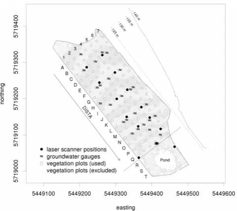
A 20 m×20 m grid for sampling and orientation purposes was established across the catchment area (Fig. 1). The data used in this study cover the sub-area between the grid-point lines A and Q as shown in Fig. 1 which amounts to ap-proximately 5 ha. The other part, the area around the pond in the lower part of the catchment, was excluded from our study since it is influenced by a high, constant water table and evolved into a semi-aquatic ecosystem with different site conditions.

For the statistical scrutiny of our hypotheses a combined data set comprising terrain surface information from terres-trial laser scanning (TLS), vegetation information from field records, soil and groundwater information was used. The data sources have different spatial and temporal resolutions. Soil samples were taken only once at the beginning of the study, vegetation records were made once every year in sum-mertime and TLS was done at seven different times between 2008 and 2011.

The above-mentioned 20 m×20 m grid points form the basic units of each analysis carried out. A spatial data fusion was thus done in order to assign the different data sources to the grid (see below). Temporally, vegetation record data were assigned to the same year’s laser scan data. Thus, dependent on the analysis of interest, the same vegetation record data were assigned to both laser scan measurements of a year. Groundwater measurements were assigned as annual means

52 1090

1091

Figure 1 1092

Fig. 1. Map of the Chicken Creek area (with Gauss–Krüger zone 5

coordinates) showing locations of the data sources (vegetation plots, laser scanner positions, groundwater gauge positions) relevant for this study. Vegetation plots are identified by “row” (A–T) and “col-umn” (1–7). In this work only rows A–Q were used. The variable DISTA as shown in the figure indicates the distance of a point from row A. Ground heights a.s.l. are given as mean values from the laser scan in September 2008 around the centre points of vegetation plots A6, F6, L6 and Q6. The height profile along row 4 is given (top right) in the map. It shows the ground elevation as obtained from the laser scans in September 2008.

to each grid point. As there was only one survey of soil prop-erties, a specific temporal assignment was not possible. Thus, for interpretation purposes they represent initial conditions and not a temporal development.

As the catchment is sloped downwards from row A to row Q, the distance of any grid point to row A is indicated as DISTA. The time since January 2005 is encoded in the variable TIME with month as yearly fractions (e.g. 6.42 for May 2011) and CALYEAR as the calendar year. In the fol-lowing text, the resulting time component of the variables used in this study is identified by the indexj and the spatial location by the indexi. In Table 1 we list all variables and indexes together with their definitions, while in Table 2 we present their summary statistics (more details below). All re-sponse variables were chosen and calculated a priori, based on considerations about ecological interpretability and plau-sibility.

2.3 Vegetation

Table 1. Names, data source and description of the variables used in this study.

Source Variable Description Unit

TLS RILLRij Proportion of laser scan cells classified as belonging to a rill related to the total amount of laser scan cells per vegetation plot

TLS RELENij Mean value of local relief energy (0.8 m radius neighbourship) m

TLS DHEIGHTij Mean ground surface elevation changes between September 2008 and May 2009, May m 2009 and April 2010, and April 2010 and February 2011. Positive values of DHEIGHT indicate an increase of the surface height indicating a net gain of substrate material in the

vegetation square, while negative values indicate a net substrate material export (erosion) from the respective square

TLS VEGHEIGHTij Mean vegetation height m

TLS VEGDENSij Mean vegetation density surrogate

TLS VEGDHij Product of VEGHEIGHTijand VEGDENSij

VEG PROPANNij Proportion of annual plant cover related to total plant cover VEG PROPHERBij Proportion of herbaceous plant cover related to total plant cover VEG PROPGRASSij Proportion of grass like plants cover related to total plant cover VEG PROPWOODij Proportion of woody plants cover related to total plant cover

VEG PROPFABij Proportion of cover of plants belonging to the Fabaceae family related to total plant cover

VEG COVTOTij Total degree of plant coverage SOIL CORGPi Percentage of organic carbon in the soil SOIL SKELCONTi Percentage of skeletal content in the soil

SOIL MSANDi Percentage of medium sand (0.2–0.63 mm) in the soil

AQ GAUGEij Mean annual groundwater level below surface m

DISTAi Distance from the row of the grid point to the row A on the catchment (see Fig. 1) m

TIMEj Time in years since January 2005, months included as fractions of years a

CALYEARj Calendar year a

TLS: derived from laser scans, available for each laser scan grid cell, aggregated for each vegetation plot. VEG: derived from the vegetation monitoring, summer of each year. SOIL: values from soil samples in 2005 at the centre of each vegetation plot. AQ: values assigned from the nearest of the groundwater gauges, yearly averages. Indices:i values for a specific location (grid point), constant over time.jvalues for points in time, spatially independent. ij values for a specific point in time, at a specific location.

point in its centre. At each plot all vascular plant species were recorded including cover estimates for each species in 30 distinct percentage classes (Zaplata et al., 2013). Bryophyte covers were estimated in the same way, distin-guishing mosses and liverworts. For this study, a time se-ries with 6 yr of annual monitoring (2006–2011) is available. The plant species were grouped by (i) lifespan according to Rothmaler (2000), but with only the two categories “an-nual” and “perennial”; (ii) life forms “grass-like”, “herb” or “wood” according to Rothmaler (2000), species of the genus Rubus which in general form woody stems were thus la-belled as “wood”; and (iii) affiliation to the Fabaceae family (“Fabaceae” versus “no Fabaceae”). Fabaceae species are of special interest, because they are the only N-fixing vascular plants found on the catchment. Other N-fixing organisms are cyanobacteria, which are part of biological soil crusts, also found at the study site (Fischer et al., 2012). However, in this context Fabaceae is the most important group by far. See Table A.1 in the Appendix for each vascular plant species’ group affiliation.

In Table 3 we summarize the covers separately for the above-mentioned groups and for all plants together. These group-wise and overall covers were obtained by summing up the single species’ covers as recorded in the field. The total

plant cover increases from an average of 2.0 % in 2006 up to 105.7 % in 2011. The latter value, being greater than 100 %, indicates an overlap of the areas covered by different species. This dramatic rise occurs rather homogeneously across the area, albeit with a slightly higher cover on its central longitu-dinal axis (Supplement Fig. S1). While from 2006 to 2008 the vascular plants (annuals and perennials) almost exclu-sively contribute to the total cover, the further increase of total cover is carried by a massive increase of the bryophytes between 2010 and 2011 (Elmer et al., 2013). The vascular plants’ cover, however, seems to stabilize between 30 and 40 % during 2009–2011.

The annual plants reach a distinct maximum cover of more than 30 % in 2009 which considerably decreases in the following years. A similar development, but with a less steep decline, can be seen for the herbaceous plants because this group largely overlaps with the annuals (Supplement Figs. S2, S3). Since 2008, Fabaceae occur with very simi-lar cover values as the annuals do. This is due to the annual species Trifolium arvense L. (Fabaceae) which is the most prominent annual species from 2008 to 2011 (cf. Zaplata et al., 2011b, Supplement Fig. S4).

Table 2. Summary statistics of the variables used in this study (see Table 1 for variable explanations). DHEIGHT, indicating a change between

subsequent years, is given always at the start year. The soil-related variables CORGP, GRAVCONT, and MSAND were only measured once in 2005. DISTA does not change with time and is presented for the time when the catchment’s establishment was completed. The variable COVTOT is shown in Table 3 together with other vegetation properties.

2005 2006 2007 2008 2009 2010 2011 variable unit min mean max min mean max min mean max min mean max min mean max min mean max min mean max

RILLR 0.00 0.10 1.00 0.00 0.09 1.00 0.00 0.10 1.00 0.00 0.16 1.00

RELEN m 0.01 0.13 1.08 0.00 0.12 1.27 0.01 0.13 1.70 0.01 0.22 2.03

DHEIGHT m −0.77 −0.03 0.39 −1.51 0.00 0.51 −0.55 0.04 0.97

VEGHEIGHT m 0.00 0.35 2.16 0.00 0.40 3.63 0.01 0.51 4.49 0.00 0.80 5.60

VEGDENS 0.01 0.38 1.00 0.01 0.37 1.00 0.01 0.38 1.00 0.00 0.37 1.00

VEGDH m 0.00 0.13 1.30 0.00 0.15 1.83 0.01 0.20 3.45 0.00 0.30 4.39

PROPANN 0.00 0.71 1.00 0.07 0.63 0.99 0.08 0.59 0.88 0.05 0.64 0.96 0.03 0.29 0.74 0.01 0.21 0.56

PROPHERB 0.32 0.81 1.00 0.34 0.80 1.00 0.18 0.69 0.94 0.13 0.70 0.94 0.15 0.42 0.84 0.09 0.29 0.67

PROPGRASS 0.00 0.19 0.68 0.00 0.19 0.66 0.06 0.28 0.59 0.01 0.13 0.86 0.03 0.13 0.44 0.01 0.07 0.57

PROPWOOD 0.00 0.00 0.08 0.00 0.00 0.05 0.00 0.01 0.15 0.00 0.01 0.34 0.00 0.02 0.61 0.00 0.02 0.50

PROPFAB 0.00 0.00 0.06 0.00 0.11 0.78 0.00 0.33 0.85 0.01 0.57 0.91 0.01 0.24 0.64 0.01 0.20 0.57

CORGP % 0.00 0.16 0.57

GRAVCONT % 0.24 15.21 25.30

MSAND % 9.65 46.91 62.43

GAUGE m 0.39 1.78 2.79 0.27 1.46 2.40 0.17 1.30 2.15 0.10 1.12 2.05 0.11 0.75 1.45 0.16 0.90 1.62

DISTA m 0.00 154.21 320.00

Table 3. Minimum, mean and maximum covers in % per plant species group and year of survey. The allocation of the single plant species

to the groups is shown in Table 14. COVTOT is the total degree of coverage by plants (see Table 1). This variable has larger values than the cover sum of annual and perennial, or grass-like, herbaceous, and woody plants, because it also includes the bryophytes.

2006 2007 2008 2009 2010 2011

variable min mean max min mean max min mean max min mean max min mean max min mean max

annual 0.0 1.5 19.5 0.5 5.1 33.4 1.5 9.1 46.6 2.3 31.5 81.7 1.4 14.7 63.0 1.3 22.0 55.6 perennial 0.0 0.6 5.6 0.1 2.9 26.9 0.8 5.3 41.7 1.5 7.7 42.7 3.6 14.3 39.2 4.3 14.8 50.9 grass-like 0.0 0.5 10.5 0.0 1.5 9.9 0.6 3.7 18.5 1.0 4.5 17.6 2.0 6.0 13.9 1.3 5.6 21.0 herbaceous 0.1 1.6 14.5 0.9 6.5 35.2 1.9 10.6 48.6 1.5 34.3 84.5 4.1 21.9 66.5 7.8 29.4 79.7 woody 0.0 0.0 0.1 0.0 0.0 0.7 0.0 0.1 1.6 0.0 0.4 6.5 0.0 1.1 20.7 0.0 1.7 40.1 Fabaceae 0.0 0.0 0.1 0.0 1.4 30.0 0.0 6.1 45.1 0.1 29.8 82.0 0.7 12.6 60.1 0.3 21.5 54.6 COVTOT 0.1 2.0 25.1 1.1 8.3 68.8 2.5 15.2 112.0 5.9 48.0 147.8 10.3 59.6 134.8 13.2 105.7 166.3

still considerably lower covers than for the annuals in 2011 (Supplement Fig. S5). On a lower level, the grass-like plants show a mostly parallel development, seeming to stabilize in 2010 and 2011, with Supplement Fig. S6 suggesting strong increases at the southeast edge (near the pond) and a slight decrease across the rest of the area. Compared to the other plant groups, the covers of woody plants seem negligible so far. However, their average cover increased exponentially and their presence on the whole area (Supplement Fig. S7) might be a precursor of their future dominance.

In order to capture the different groups’ relative domi-nance and to eliminate the time trend which is inherent in the absolute cover values, we related their covers for each grid point and each observation to the respective total plant cover COVTOT for further analysis. This resulted in the proportions of cover for annual plants (PROPANN), grass-like plants (PROPGRASS), woody plants (PROPWOOD) and Fabaceae family (PROPFAB) (cf. Tables 1, 2). As Ta-ble 2 shows, the herbaceous plants are the dominating vascu-lar plants throughout the observation period, however with a pronounced decrease of their share from between 0.7 and 0.8 down to about 0.4 and 0.3 in 2010 and 2011. Annual plants follow the same pattern, albeit on a slightly lower level (cf. Supplement Figs. S8, S9). Grass-like plants increase their

share from 0.2 to almost 0.3 in 2008. After that, they also drop down, but by far not as dramatically as observed for the annuals and herbaceous plants (cf. Supplement Fig. S10). The Fabaceae, almost not present in 2006, extend their share, starting from the area’s western part (Supplement Fig. S11), up to nearly 0.6 in 2009 and drop – in line with the annuals – back to 0.2 in 2011. The low shares of all these groups in 2010 and 2011 come from the above-mentioned vast increase of bryophyte covers. Only the woody plants’ share of the to-tal cover keeps steadily increasing, albeit on a very low level so far (cf. Supplement Fig. S12).

2.4 Soil and groundwater

After completion of the catchment construction, soil sam-ples were taken at each grid point at a depth of 0–30 cm be-tween October 2005 and April 2006 (see Fig. 1). The samples were air-dried, passed through a 2 mm mesh and analysed for pH (water extract, Beckmann pH34 glass electrode and WTW pH537), electrical conductivity (EC, Hanna HI 8733 and WTW LF537), texture (sieving and sedimentation pro-cedure with Köhn pipette method), total content of carbon (CT), nitrogen (NT) and sulfur (ST, elementar analyser Vario

or-ganic carbon (Corg, calculated as difference CT–CaCO3-C)

content (Sparks, 1996; Dane and Topp, 2002).

We assumed the soil data from a grid point being valid for the whole vegetation square. Variables that turned out to be promising for this study from a theoretical point of view as well as in visual exploratory data analyses were the percentage of Corg(CORGP), the percentage of gravel

con-tent (GRAVCONT), and MSAND, the percentage of medium sand (see Tables 1, 2). Hereby, the gravel fraction of a soil is defined by grain sizes of more than 2 mm. Corg– mostly

from fossil sources – was present in the initial situation, al-beit with low concentrations only (Risse-Buhl et al., 2013). These generally low concentrations of CORGP show consid-erable variation between 0 and almost 0.6 % (Table 2). Spa-tially, CORGP is not evenly distributed, higher concentra-tions are found in the south-west half of the area (Supplement Fig. S13). Mean gravel content (GRAVCONT) is about 15 % (Table 2) with a slight tendency towards higher values again in the south-west zone (Supplement Fig. S13). At an average of 47 % MSAND shows a homogeneous spatial distribution across the catchment (Table 2, Supplement Fig. S13).

A total of 21 groundwater gauges were initially installed across the catchment. Nine of them were equipped with pres-sure transducers to register groundwater levels automatically. The levels at the other gauges were measured manually ev-ery two weeks. During the following years, five additional groundwater gauges were installed. The positions of all 26 gauges can be taken from Fig. 1. See Biemelt et al. (2010) and Supplement Fig. S14 for more details. We simply at-tributed the mean annual distance of the groundwater level from the surface (variable GAUGE, see Table 1) from the nearest measurement shaft to each grid point, with an aver-age distance of 19 m and maximum distance of 53 m from a square midpoint. We used that simple method because no complex assumptions are made as is the case for any interpo-lation method.

Since 2006, GAUGE shows a declining trend from on av-erage 1.8 down to 0.9 m in 2011, indicating rising groundwa-ter levels over time. Their spatial distribution (Supplement Fig. S14) is homogeneous in the beginning with higher lev-els only in the lowest part (south-east) with a slight tendency towards drier conditions at the south-west edge developing during the observation period.

2.5 Terrestrial laser scans

We used a terrestrial laser scanner (mod. Riegl LMS Z420i) in last target mode to measure 3-D ground surface and veg-etation height and density simultaneously. In order to keep the impact on the catchment at a minimum, we only mea-sured from 13 permanently fixed scan positions (Fig. 1), each geo-referenced with 30 DGPS-fixed points (DGPS, differen-tial global positioning system), which allowed us to keep the standard deviation of the geo-referencing error below 2.5 cm.

The scan positions were spatially arranged in a way that allowed us to maintain a horizontal measurement resolution of at least 10 cm×10 cm at a hypothetical horizontal ground surface. Given the limited number of scan positions, this was only possible by mounting the laser scanner on a portable 6 m tower. This height is sufficient for achieving the desired minimum resolution but not too high in order to hit existing vegetation mainly from more lateral and not so much from vertical directions. This is important, because vertically ori-ented vegetation like grasses is more likely detected from the side than from above and the side view is better suited to detect vegetation layers under emerging woody plants. See the method comparison by Schneider et al. (2012) for more technical details.

We conducted seven area-wide laser scan campaigns be-tween 2008 and 2011 (September 2008, Mai 2009, Au-gust 2009, April 2010, October 2010, February 2011, and May 2011). Although it was not easy to find appropriate time windows (for such a campaign several days with clear weather and low wind are required) the measurements were timed so that at least in the years 2009 and 2010 roughly the catchment’s state at the beginning and the end of the grow-ing season could be covered. With our scans we covered the whole catchment amounting to 6 ha altogether.

The raw laser scan data are three-dimensional point clouds, each point indicating the position where the laser beam hit an object. In order to separate vegetation from ground surface we divided the covered area into about 200 000 0.5 m×0.5 m grid cells. On each cell we extracted the minimum vertical coordinate from the point cloud and as-sumed it to best represent the ground surface level. Our esti-mate for vegetation height on such a cell is the vertical range of point coordinates, i.e. maximum minus minimum vertical coordinate. As a proxy for vegetation density on each cell, we took the median vertical coordinate (with the estimated ground level being zero) divided by the estimated vegeta-tion height. This results in a number between 0 and 1. Values near 1 would indicate a high density, because the laser signal will be more often reflected in higher regions if vegetation is dense, resulting in a median nearer the maximum height and for less dense vegetation more reflections are measured at the ground, shifting the median lower. Values near zero result from a small median compared to vegetation height, thus indicating the obvious high penetrability when density is low. We also calculated the product of vegetation height and vegetation density, which could serve as a rough proxy for biomass.

following form:

z=a·x+b·y+c+ε, (1)

witha,b,cbeing parameters to be estimated andε repre-senting the error term. Equation (1) thus represents a plane that after fitting can be interpreted as a smoothed descrip-tion of the terrain surface in the cell of interest’s proximity defined by the 6 m radius as explained above. If the actual ground levelzof the central cell is more than 5 cm lower than the one estimated from Eq. (1), then this cell is assumed to belong to a rill. Visual comparisons with aerial photographs from the catchment show a good agreement with this rill de-tection method.

In addition to this 6 m neighbour analysis, we used the same method with a 0.8 m radius around the cell of inter-est and calculated the difference between the greatinter-est and the smallest vertical deviation from the regression plane. This can be interpreted as a description of relief energy in the near-est neighbourhood. This potential energy is used as an indi-cator if the cell is located on a jagged or smooth surface and thus how large the influence of surface runoff events might be or how likely a successful seed deposition may happen.

Changes of the ground surface level inform about erosion and deposition processes. For each cell we calculated the dif-ference between the surface level at a given and a previous survey, requesting a survey-to-survey time distance closest to one year. Negative numbers, i.e. decreasing surface levels, indicate erosion while positive numbers indicate deposition. For our analysis the changes were always attributed to the first of the two surveys, in other words to the status before the change.

To each 20 m×20 m grid point we attributed every laser scan grid cell with its midpoint inside the corresponding 5 m×5 m vegetation square and used only those cells there-after. This resulted in about 100 laser scan cells per vegeta-tion square and implied two opvegeta-tions for data evaluavegeta-tion. First is the extraction and evaluation of sum and mean values from the laser scan data, one number per vegetation square, such as surface roughness or percentage of rill cells. Second is an analysis on the level of single laser scan grid cells. However, preliminary analyses showed that the latter tended to be less revealing than the former while consuming disproportional computing time. Thus, we focussed on the former, more ag-gregated option.

For further analysis, the following variables were calcu-lated from the laser scan data, resulting in one number per grid point and survey (cf. Table 1): VEGHEIGHT and VEG-DENS are the mean vegetation height and the mean vegeta-tion density of all laser scan grid cells on a vegetavegeta-tion square. VEGHD is their product. RILLR is the proportion of rill cells as defined above on a given vegetation square while RELEN is the average relief energy of all laser scan cells on one vegetation square. DHEIGHT represents the average surface height change of all laser scan cells belonging to a given veg-etation square.

On average VEGHEIGHT more than doubles from 2008 to 2011 (0.35 to 0.80 m, Table 2). The highest vegetation concentrates in the southern and south-west part of the catch-ment in 2011 (Supplecatch-ment Fig. S15). The vegetation density, VEGDENS, on average remains constant during the observa-tion period, albeit with changing spatial distribuobserva-tion (Table 2, Supplement Fig. S16). Its overall constancy despite increas-ing heights confirms its adequacy for expressincreas-ing vegetation density independent from plant size. Accordingly VEGDH, the product of both, doubles from 2008 to 2011 in a similar way as VEGHEIGHT, being greatest in the southern corner and the east side of the area, where both, height and density are high (Table 2, Supplement Fig. S17).

The average proportion of rill cells per vegetation square, RILLR, does only slightly increase from 0.10 to 0.16 from 2008 to 2011 (Table 2). Being concentrated on the north-ern, western and southern edges of the investigated area from 2008 to 2010 a redistribution towards the south-eastern part of the catchment seems to have occurred between 2010 and 2011 (Supplement Fig. S18). Similar to RILLR, the local re-lief energy, RELEN, stays nearly constant between 0.12 and 0.13 from 2008 to 2010 but almost doubles from 2010 to 2011 accompanied with a spatial redistribution of the high-est values towards the eastern edge (Table 2, Supplement Fig. S19). The surface height change, DHEIGHT, undergoes a reversion during the observation time span. In average, one vegetation square lost 3 cm of terrain height between 2008 and 2009, from 2009 to 2010 there was on average no change, and from 2010 to 2011 we observe an average surface height increase of 4 cm (Table 2). A spatial view, as provided in Supplement Fig. S20, shows that erosion first dominated throughout the catchment, being strongest at the western edge. Later we observe a central ridge where terrain height slightly increases while erosion weakens but contin-ues along the western and the eastern edges. From 2010 to 2011 deposition dominates the whole area, being strongest in the north-western part.

2.6 Statistical evaluation

spa-tial correlation between vegetation squares did not improve our models.

The core of a GLMM in the context of this study is a linear predictor functionηof the following form:

η(X1ij, . . . , Xq ij)=α+β1·X1ij+. . .+βq·Xq ij+ai (2) ai∼N (0, σa2),

whereX1. . . Xq, is a set ofq explanatory variables. The

in-dices i and j denote the jth observation on the ith veg-etation square. α and β are regression parameters and ai

is a vegetation-square specific random effect. In case of a GAMM, the predictor function enlarges to

η X1ij, . . . , Xq ij, K1ij, . . . , Kn ij

=α+β1·X1ij

+. . .+βq·Xq ij+f1 K1ij+. . .+fn Kn ij+ai,

(3)

where, in addition,K1. . . Kn is a set ofnexplanatory

vari-ables, andf1. . . fnis a set of nonparametric smoother

func-tions (cf. Zuur et al., 2009).

The way, thatηis transformed into an expected value µij

for the actual response variable Yij is defined by the link

functiong.

g µ_ij=η X1ij, . . . , Xq ij, K1ij, . . . , Kn ij

(4) If the response variableYij is assumed to be normally

dis-tributed (Yij∼N (µij, σ2)) then the usual link function is

identity:

µ_ij=η X1ij, . . . , Xq ij, K1ij, . . . , Kn ij.

(5) This is the first of three options we used in this study.

In cases whereYij was proportional data with a tendency

towards over-dispersion, a quasi-binomial distribution forYij

withvar(Yij)=τ·µij·(1−µij)and the dispersion parameter τ not being fixed to 1 and a logit link

ln µij 1−µ_ij

!

=η X1ij, . . . , Xq ij, K1ij, . . . , Kn ij (6)

was used. WhenYij>0, the assumption of a gamma

distri-bution forYij withvar(Yij)= µ2

ij

ν andνbeing the dispersion

parameter turned out to be useful in combination with a log-arithmic link:

ln µ_ij=η(X1ij, . . . , Xq ij, K1ij, . . . , Kn ij). (7)

Promising explanatory variables for each single regres-sion analysis were pre-selected by theoretical considerations and, as proposed by Zuur et al. (2009), based on descriptive exploratory data analyses such as pair-plots and variance-inflation factors. If plausibility, visual data inspections or residual plots suggested (partly) nonlinear relationships, a GAMM was chosen instead of a GLMM. In each analysis,

we started with the full set of pre-selected explanatory vari-ables, leaving them out stepwise, by AIC comparison and re-fitting each time (Zuur et al., 2009). Model assumptions were confirmed by graphical displays.

Presenting the most important results of a model fit is straightforward for a GLMM (Eq. 2). Presenting the linear parameters’β1,. . .,βqestimates together with their standard

errors and significance levels is standard. In the case of a GAMM, this can be done in exactly the same way for the linear components of the model. However, the components which are expressed by nonparametric smoother functions (f1(K1ij),. . .,fn(Knij)in Eq. 3) can only be displayed

visu-ally. Thus, for a GAMM, a table is needed for presenting the linear components and a diagram is needed for each compo-nent that is represented by a smoother function.

In order to scrutinize H1, “do the initial geomorphological and substrate characteristics determine the surface’s struc-ture and properties of the terrain?”, we investigated several response variables (see Table 1):

– RILLR: the proportion of rill cells per vegetation square and measurement. As RILLR represents pro-portional data, the quasibinomial distribution with logit link was used.

– RELEN: the mean value of the local relief energy of all laser scan cells belonging to one vegetation square. As-suming a gamma distribution combined with the log-arithmic link matched the data well from a theoretical point of view and yielded good model fits for this re-sponse variable.

– DHEIGHT: the ground’s height change (see Table 1 for details) was investigated with a regression model that assumes normal distribution of the response vari-able and uses the identity link.

Due to the definition of H1 we did not include any vegeta-tion properties as explanatory variables in these analyses.

In the context of H2, asking if surface and substrate char-acteristics determine the plant species groups to be found ini-tially, the following set of vegetation properties was chosen as response variables (see Table 1):

– PROPANN: the portion of annual plants related to the total coverage per vegetation square and survey. – PROPHERB: same for the portion of herbaceous

plants.

– PROPGRASS: same for grass including sedges.

– PROPFAB: same for plants belonging to the nitrogen-fixing Fabaceae family.

P. Biber et al.: Relationships between substrate, surface characteristics, and vegetation 8291

53 1094

Figure 2

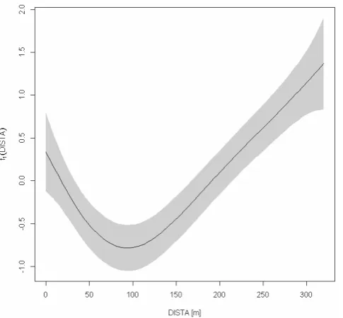
1095 Fig. 2. Nonlinear effect of a vegetation square’s distance from grid-row A (DISTA) on the portion of rill cells (RILLR) (see Eq. 8). Shaded: 95 %-confidence area.

For all these proportions, assuming quasi-binomial distri-bution and using a logit link turned out to be the best option. In addition, we also used two laser-scanned vegetation prop-erties as response variables:

– VEGHEIGHT and VEGDENS: the mean vegetation height and vegetation density per vegetation square and survey.

The former was investigated assuming normal distribution and using the identity link while for the latter quasi-binomial distribution with logit link was applied.

For testing H3, if increasing density of vegetation reduces the erosion, we used DHEIGHT: the laser-scanned surface height changes as a response variable.

We did so in the same way as for H1, but tested sev-eral ways of including the laser-scanned vegetation proper-ties VEGHEIGHT and VEGDENS as additional explanatory variables. The other explanatory variables were those that showed significance in the context of H1.

The overall important components of temporality and spa-tiality are included in the variables TIME and DISTA. The final models with the final set of explanatory variables are shown in the results section. Table 1 explains all variables used in this study, and Table 2 presents their means, minima and maxima for each observation year.

For all statistical evaluations we used the free software R version 2.15.1 (R Core Team, 2012), namely the package mgcv (Wood, 2006).

54 1096

Figure 3

1097 Fig. 3. Nonlinear effect of a vegetation square’s distance from grid-row A (DISTA) on the local relief energy (RELEN) (see Eq. 9). Shaded: 95 %-confidence area.

3 Results

3.1 Influence of geomorphological and substrate char-acteristics on surface structure (H1)

The final model for describing the dependency of the por-tion of rill cells, RILLR, was a GAMM with logit link (cf. Sect. 2.3, Eqs. 3, 6):

ln

_E(RILLR ij)

1−E(RILLRij)

=α+β₁·CORGPi+β₂·GAUGEij+

β3·TIMEj+β4·CORGPi·TIMEj+f1(DISTAi)+ai. (8) The indicesiandj, and the random effecta have the same meaning as in Eq. (2), andE(RILLR) represents the expected value of RILLR. CORGP is the percentage of organic carbon in the soil, GAUGE is the mean annual groundwater level in m below surface, andf1(DISTA) is a smoother function that

represents the effect of DISTA (see Table 1). All explanatory variables show highly significant (p <0.001) effects.

Figure 2 shows the effect of DISTA. Clearly there is a gen-eral trend of more likely finding rills the more one moves fur-ther downslope, however with a minimum between 50 and 150 m from row A. Table 4 lists the parameter estimates for

αandβ1,. . .,β4. The parameters for the variables CORGP,

GAUGE, and TIME are greater than 0, indicating that the probability of encountering rills increases with the percent-age of organic carbon (as measured in 2005), a lower annual groundwater level (higher GAUGE) and with time. However, there is also a significant interaction that indicates the influ-ence of CORGP weakens with time.

how-Table 4. Parameter estimates and significances for the model estimating the portion of rill cells (RILLR) as shown in Eq. (8). Significance

levels: ***:p <0.001, **:p <0.01, *:p <0.05. The variance of the random effectain Eq. (8) is 0.5456. Trend: qualitative illustration of linear predictor variables’ significant influences.↑,↓: RILLR increases (decreases) with increasing values of the respective predictor variable.

Variable Trend Parameter Estimate Std. Error Significance

α −8.1121 0.5397 ***

CORGP ↑ β1 10.4752 2.0661 ***

GAUGE ↑ β2 1.0374 0.1753 ***

TIME ↑ β3 0.8624 0.0820 ***

CORGP*TIME ↓ β4 −1.7634 0.3555 ***

f1(DISTA) Nonparametric smoother See Fig. 2 ***

Table 5. Parameter estimates and significances for the model estimating the local relief energy (RELEN) as shown in Eq. (9). Significance

levels: ***:p <0.001, **:p <0.01, *:p <0.05. The variance of the random effectain Eq. (9) is 0.1119. Trend: qualitative illustration of linear predictor variables’ significant influences.↑,↓: RELEN increases (decreases) with increasing values of the respective predictor variable.

Variable Trend Parameter Estimate Std. Error Significance

α −5.5417 0.2758 ***

CORGP ↑ β1 5.7311 1.1252 ***

GAUGE ↑ β2 0.5085 0.0894 ***

TIME ↑ β3 0.5726 0.0434 ***

CORGP*TIME ↓ β₄ −1.0869 0.2031 ***

f1(DISTA) Nonparametric smoother See Fig. 3 ***

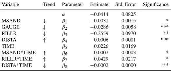
Table 6. Parameter estimates and significances for the model estimating surface height change (DHEIGHT) as shown in Eq. (10). Significance

levels: ***:p <0.001, **:p <0.01, *:p <0.05. The variance of the random effectain Eq. (10) is 0.0002. Trend: qualitative illustration of linear predictor variables’ significant influences.↑,↓: DHEIGHT increases (decreases) with increasing values of the respective predictor variable. Thus,↓indicates a tendency towards erosion while↑indicates trends that counteract erosion.

Variable Trend Parameter Estimate Std. Error Significance

α −0.0414 0.0825

MSAND ↓ β1 −0.0031 0.0015 *

GAUGE ↓ β2 −0.0286 0.0058 ***

RILLR ↓ β3 −0.2559 0.0970 **

DISTA ↑ β4 0.0006 0.0001 ***

TIME β5 0.0226 0.0169

MSAND*TIME ↑ β6 0.0007 0.0003 *

RILLR*TIME ↑ β7 0.0429 0.0217 *

DISTA*TIME ↓ β8 −0.0002 0.0000 ***

ever, due to the logarithmic link function the left-hand side is different:

ln E RELENij=α+β1·CORGPi+β2·GAUGEij+ β3·TIMEj+β4·CORGPi·TIMEj+f1(DISTAi)+ai. (9)

The results as presented in Table 5 and Fig. 3 show a strong affinity between the local relief energy and the rill probabil-ity. Again, relief energy generally increases with increasing DISTA, however with a minimum at about 100 m from row A (Fig. 3). Relief energy also increases with CORGP (Table 5), lower groundwater levels (higher GAUGE) and, expectedly, increases with TIME (parametersβ1, . . . ,β3>0), however

the negative value obtained forβ4shows a weakening

influ-ence of CORGP with time.

The change of the surface height, DHEIGHT, in relation to non-vegetation variables only, yielded a final model of the following GLMM structure:

E DHEIGHTij=α+β1·MSANDi+β2·GAUGEij

+β3·RILLRij+β4·DISTAi+β5·TIMEj

+β6·MSANDi·TIMEj+β7·RILLRij·TIMEj

+β8·DISTAi·TIMEj+ai.

(10)

55 1098

Figure 4 1099

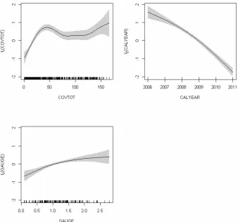
Fig. 4. Nonlinear effects of the total degree of coverage (COVTOT), calendar year (CALYEAR), and groundwater level (GAUGE) on the

proportion of annual plants (PROPANN) (see Eq. 11). Shaded: 95 %-confidence area.

Table 7. Parameter estimates and significances for the model estimating the proportion of annual plants (PROPANN) as shown in Eq. (11).

Significance levels: ***:p <0.001, **:p <0.01, *:p <0.05. The variance of the random effectain Eq. (11) is 0.1594. Trend: qualitative illustration of linear predictor variables’ significant influences.↑,↓: PROPANN increases (decreases) with increasing values of the respective predictor variable.

Variable Trend Parameter Estimate Std. Error Significance

α 0.2551 0.0868 **

CORGP ↓ β1 −1.7067 0.4431 ***

f1(COVTOT) Nonparametric smoother See Fig. 4 ***

f2(CALYEAR) Nonparametric smoother See Fig. 4 ***

f3(GAUGE) Nonparametric smoother See Fig. 4 ***

0.63 mm) in the substrate (as measured in 2005). The pa-rameter estimates and significances are listed in Table 6. Significances are partly weaker than in the models shown above. The effect of MSAND (β1<0) means that more

ma-terial (volume) erodes at places where more medium sand was found in 2005. Lower groundwater levels are connected with greater material export (β2<0), the more rills we find,

the more material is exported (β3<0). There is a weak, but

highly significant tendency towards a surface height increase – indicating deposition effects – with increasing DISTA (β4>0) while time has no significant isolated effect,

how-ever the analysis reveals significant time effects in interac-tion with other variables. Parameterβ6, being significantly

greater than 0 indicates that the above-mentioned effect of MSAND weakens with time, and the same is true for the effect of RILLR (β7>0). A reverse effect is observed for

DISTA in interaction with time (β8<0), which describes

56 1100

Figure 5 1101

Fig. 5. Nonlinear effects of the total degree of coverage (COVTOT), calendar year (CALYEAR), and groundwater level (GAUGE) on the

proportion of herbaceous plants (PROPHERB) (see Eq. 12). Shaded: 95 %-confidence area.

Table 8. Parameter estimates and significances for the model estimating the proportion of herbaceous plants (PROPHERB) as shown in

Eq. (12). Significance levels: ***:p <0.001, **:p <0.01, *:p <0.05. The variance of the random effectain Eq. (12) is 0.0855. Trend: qualitative illustration of linear predictor variables’ significant influences.↑,↓: PROPHERB increases (decreases) with increasing values of the respective predictor variable.

Variable Trend Parameter Estimate Std. Error Significance

α 0.6254 0.0685 ***

CORGP ↓ β1 −0.9162 0.3481 **

f1(COVTOT) Nonparametric smoother See Fig. 5 ***

f2(CALYEAR) Nonparametric smoother See Fig. 5 ***

f3(GAUGE) Nonparametric smoother See Fig. 5 ***

3.2 Influence of surface and substrate characteristics on vegetation structure (H2)

With the proportion of annual plants, PROPANN, as the re-sponse variable the following final model resulted (GAMM with logit-link):

ln₁₋E_E(PROPANNij) (PROPANNij)

=α+β1·CORGPi+f1 COVTOTij

+f2 CALYEARj+f3 GAUGEij+ai.

(11)

With β1< 0, Table 7 shows a negative correlation

be-tween CORGP and the proportion of annual plants. The

Table 9. Parameter estimates and significances for the model estimating the proportion of grasses (PROPGRASS) as shown in Eq. (13).

Significance levels: ***:p <0.001, **:p <0.01, *:p <0.05. The variance of the random effectain Eq. (13) is 0.1489.

Variable Parameter Estimate Std. Error Significance

α −1.9460 0.0783 ***

CORGP β1 0.7366 0.3960 p=0.0633

f1(COVTOT) Nonparametric smoother See Fig. 6 ***

f2(CALYEAR) Nonparametric smoother See Fig. 6 ***

Table 10. Parameter estimates and significances for the model estimating the proportion of woody plants (PROPWOOD) as shown in

Eq. (14). Significance levels: ***:p <0.001, **:p <0.01, *:p <0.05. The variance of the random effectain Eq. (14) is 3.1987. Trend: qualitative illustration of linear predictor variables’ significant influences.↑,↓: PROPWOOD increases (decreases) with increasing values of the respective predictor variable.

Variable Trend Parameter Estimate Std. Error Significance

α −1118.7522 98.9546 ***

COVTOT ↓ β1 −0.0119 0.0018 ***

CALYEAR ↑ β2 0.5542 0.0493 ***

A very similar final model resulted for PROPHERB, the proportion of herbaceous plants (GAMM with logit link).

ln E(PROPHERBij) 1−E(PROPHERBij)

=α+β1·CORGPi+f1 COVTOTij

+f2 CALYEARj

+f3 GAUGEij

+ai

(12)

The effects observed for PROPHERB are virtually the same as obtained for annual plants (Fig. 5, Table 8), an op-timum pattern for COVTOT, a decreasing curve for the cal-endar year and a saturation curve for the groundwater level, and a negative correlation with CORGP.

The scrutiny of the proportion of grasses (PROGRASS) yielded an even simpler model:

ln E(PROPGRASSij)

1−E(PROPGRASSij)

=α+β1·CORGPi

+f1 COVTOTij

+f2 CALYEARj

+ai.

(13)

Compared to the herbaceous plants, the grasses show an opposing trend. Even though the effect of CORG is just not significant (p=0.0633, Table 9), the grasses seem to be connected to places with higher organic carbon content in the soil. As Fig. 6 shows, the coverage of grasses decreases strongly with the total degree of coverage (COVTOT), while it increases with the calendar year. This indicates that grass-like plants preferentially establish where the total cover is not too high.

For the proportion of woody plants (PROPWOOD) a sim-ple GLMM resulted:

ln E(PROPWOODij) 1−E(PROPWOODij)

=α+β1·COVTOTij

+β2·CALYEARj+ai.

(14)

Only two explanatory variables show a significant rela-tionship in this context. Trivially, the proportion of woody

57 1102

Figure 6

1103 Fig. 6. Nonlinear effects of the total degree of coverage (COV-TOT), and calendar year (CALYEAR), on the proportion of grasses (PROPGRASS) (see Eq. 13). Shaded: 95 %-confidence area.

plants increases with time (CALYEAR). Less expectedly, the probability of finding woody plants decreases as the total coverage on a vegetation square increases (Table 10).

The final model for the proportion of Fabaceae (PROP-FAB) resulted in the following structure:

ln E(PROPFABij) 1−E(PROPFABij)

=α+β1·GAUGEij+f1 COVTOTij

+f2 CALYEARj+f3(GRAVCONTi)+ai,

(15)

with GRAVCONT representing the soil’s gravel content in percent as measured in 2005.

As Table 11 shows, there is a positive correlation between lower groundwater levels and the occurrence of Fabaceae (β1>0). Up to gravel contents of 10 % and up to total

58 1104

Figure 7 1105

Fig. 7. Nonlinear effects of the total degree of coverage (COVTOT), calendar year (CALYEAR), and gravel content (GRAVCONT), on the

proportion of Fabaceae (PROPFAB) (see Eq. 15). Shaded: 95 %-confidence area.

Table 11. Parameter estimates and significances for the model estimating the proportion of Fabaceae (PROPFAB) as shown in Eq. (15).

Significance levels: ***:p <0.001, **:p <0.01, *:p <0.05. The variance of the random effectain Eq. (15) is 0.2288. Trend: qualitative illustration of linear predictor variables’ significant influences.↑,↓: PROPFAB increases (decreases) with increasing values of the respective predictor variable.

Variable Trend Parameter Estimate Std. Error Significance

α −2.6636 0.1723 ***

GAUGE ↑ β1 0.8693 0.1301 p=0.0633

f1(COVTOT) Nonparametric smoother See Fig. 7 ***

f2(CALYEAR) Nonparametric smoother See Fig. 7 ***

f3(GRAVCONT) Nonparametric smoother See Fig. 7 ***

VEGHEIGHT, the mean vegetation height, as obtained from laser scans was described with the following model:

E VEGHEIGHTij=α+β1·COVTOTij+β2·GAUGEij

+f1 CALYEARj+f2(DISTAi)+ai.

(16) Figure 8 (left) shows that vegetation height increases with time, expectedly in an exponential pattern as it is typical for initial growth processes. The same figure (Fig. 8, right) re-veals a clear trend of increasing vegetation height with the

distance from grid-row A. Depth to groundwater table and coverage degrees are positively correlated with vegetation height (β1>0,β2>0, Table 12).

No significant relations of other variables with the laser-scanned vegetation density, VEGDENS, could be identified. 3.3 Influence of vegetation structure on surface

structure (H3)

Table 12. Parameter estimates and significances for the model estimating the laser-scanned vegetation height (VEGHEIGHT) as shown in

Eq. (16). Significance levels: ***:p <0.001, **:p <0.01, *:p <0.05. The variance of the random effectain Eq. (16) is 0.0074. Trend: qualitative illustration of linear predictor variables’ significant influences.↑,↓: VEGHEIGHT increases (decreases) with increasing values of the respective predictor variable.

Variable Trend Parameter Estimate Std. Error Significance

α 0.3851 0.0367 ***

COVTOT ↑ β1 0.0007 0.0003 *

GAUGE ↑ β2 0.0879 0.0301 **

f1(CALYEAR) Nonparametric smoother See Fig. 8 ***

f2(DISTA) Nonparametric smoother See Fig. 8 ***

Table 13. Parameter estimates and significances for the model estimating surface height change (DHEIGHT) as shown in Eq. (17).

Sig-nificance levels: ***:p <0.001, **:p <0.01, *:p <0.05. The variance of the random effectain Eq. (17) is 0.0006. Trend: qualitative illustration of linear predictor variables’ significant influences.↑,↓: DHEIGHT increases (decreases) with increasing values of the respec-tive predictor variable. Thus,↓indicates a tendency towards erosion while↑indicates trends that counteract erosion.

Variable Trend Parameter Estimate Std. Error Significance

α −0.0427 0.0253

MSAND ↓ β1 −0.0024 0.0004 ***

GAUGE ↓ β2 −0.0392 0.0032 ***

RILLR ↓ β3 −0.0215 0.0072 **

DISTA ↑ β4 0.0004 0.0000 ***

TIME ↑ β5 0.0189 0.0038 ***

MSAND*TIME ↑ β6 0.0007 0.0000 ***

RILLR*TIME ↑ β7 0.1075 0.0016 ***

DISTA*TIME ↓ β8 −0.0002 0.0000 ***

f1(VEGHD, TIME) Nonparametric smoother See Fig. 9 ***

DHEIGHT, with soil and surface variables, but added differ-ent combinations of the laser-scanned VEGHEIGHT, VEG-DENS, and TIME, all referring to the beginning of the period during which DHEIGHT occurred. We found that including the product of VEGHEIGHT * VEGDENS=VEGDH in interaction with time yielded the best model:

E DHEIGHTij

=α+β1·MSANDi+β2·GAUGEij

+β3·RILLRij+β4·DISTAi+β5·TIMEj

+β6·MSANDi·TIMEj+β7·RILLRij·TIMEj

+β8·DISTAi·TIMEj+f1 VEGDHij,TIMEj

+ai.

(17)

Compared to the model without vegetation data as ex-planatory variables (Eq. 10, Table 6), the parameter estimates forβ1,. . .,β8are very similar (Table 13), thus, there is no

contradiction between this and the other model. However, the nonlinear vegetation effect pronouncedly shows a vegetation impact that counteracts erosion. The higher and denser the vegetation (i.e. the greater VEGDH), the stronger this effect, which also changes with time (Fig. 9). In the first observation period (starting September 2008) the correlation is somewhat weak and almost linear but in the following two periods, the curve becomes more and more bent upwards, the VEGDH value where the bend starts moving down to smaller VEGDH values from the second to the third observation period. This

indicates that even with the same VEGDH values the stabi-lizing effect of vegetation increases with time.

4 Discussion

Surface structure in the study area is mainly influenced by geomorphological characteristics. The slope degree of the area is not the same throughout the area, but shows a max-imum in the lower part (rows L to P in Fig. 1). This is re-flected (or at least indicated) by the pronounced and partly nonlinear effects of the downhill distance from grid-row A (DISTA) on the frequency of rills (RILLR), the local re-lief energy (RELEN), and the ground surface height change (DHEIGHT). The pronounced minima for the downhill dis-tance effect (DISTA) for the rill frequency and the local relief energy (Figs. 2, 3) seem to indicate a special local situation: they are located just downhill an area where, due to the con-struction works of the catchment, many rills take a perpen-dicular course to the main slope direction (cf. Schaaf et al., 2013, Supplement Figs. S21, 22, 23).

signif-icant effects of the rill frequency (RILLR) and the interaction effect of the downhill position (DISTA) with time.

Although the portion of organic carbon (CORGP) is strongly correlated with rill intensity, it seems most likely that this parameter is a proxy for the general substrate prop-erties. The same could be true for parameter MSAND. Ac-cording to Gerwin et al. (2010), CORGP strongly correlates with clay content. In general, soil texture in the western part of the catchment is dominated by loamy sands, whereas in the eastern part pure sands dominate. These differences are reflected in the spatial extent and form of the erosion gullies being narrower and deeper in the western part, but shallower and wider in the eastern part (Schaaf et al., 2012). Thus, in general, our results indicate positive feedback processes gov-erning rill formation whereby, however, different rill types evolve on substrates with different properties.

Surface runoff dominated catchment hydrology at least in the early years, resulting in gully formation and transport of large sediment amounts that were deposited in the lower part of the hill slope and in the pond (Schaaf et al., 2012). While doing so surface runoff and erosion transported mainly finer textured material, resulting in even coarser texture at the up-hill surface substrates. This probably explains the decreas-ing influence of the substrate proxy variables CORGP and MSAND with time.

Besides such transport effects, the weakening effects of initial surface and soil properties with time reflect the in-creasing influence of vegetation coverage (see H3).

In summary, our results strongly support H1. Geomorphol-ogy (slope degree) and substrate properties like grain size distribution and resulting differences in groundwater levels affect the system strongly and in turn result in fundamental changes in geomorphology all over the area, but with main effects where the slope degree is highest. The developing vegetation cover, however, reduces the influence of these fac-tors in the course of time, leading to an increasing conserva-tion of the structures that developed at the very beginning.

Some of our results concerning the influence of surface and substrate characteristics on vegetation structure (H2) match basic assumptions of successional theory such as the decrease of annuals as well as the increase of grasses and especially woody species in the course of time (Cowles, 1899), and the general increase of vegetation height over time (Prach et al., 1997). Despite a scientific history of well over a century (Cutler, 2010) even this is noteworthy. Little effort has been made to integrate and synthesize the large number of case studies in succession to obtain a coherent generalized understanding. This is certainly due to the fact that rarely comprehensive spatial and temporal data on abiotic and bi-otic aspects of succession are collected. There are studies in the large body of literature which superbly meet a high temporal resolution but with only a very small spatial cover-age (e.g. Rebele, 1992). Projects exclusively using chronose-quences (probably the most) lack the spatial coverage for a quantitative analysis on vegetation change, both, in the sense

of spatial patterns over time and in the sense of temporal pattern in space (Baasch, 2010). Still vast uncertainty exists about process interactions within the plant community (e.g. dispersal, competition) to processes linking the community to its environment (e.g. soil property dynamics) during suc-cession. In view of the above, a particular contribution of H2 and our study is the detailed integration of biotic and abiotic aspects of succession with both temporal and spatial data.

Annual species – most of them being pioneers – were pref-erentially and expectedly found at places with less organic carbon, which means with low water and nutrient storage ca-pacities (as mentioned before organic carbon might act as a proxy for general substrate properties), and lower groundwa-ter levels. It was found also in a low-pH system that partic-ularly resource-limited places were almost exclusively colo-nized by pioneers (Baasch, 2010).

In line with basic assumptions, the annual species’ por-tion decreases with time (Fig. 4). However, during the first years of the succession two annual species (Conyza canaden-sis, Trifolium arvense) were dominant (Zaplata et al., 2011b) and hence their portion increases with increasing vegetation cover (COVTOT) but does not change with COVTOT val-ues beyond 50 % (Fig. 4). The existence of a succession phase governed by Trifolium arvense (Fabaceae) in 2008– 2009 means, that many (adjacent) vegetation plots had simi-lar covers of this plant species (Zaplata et al., 2013). The “op-timum” shortly before COVTOT=50% (Fig. 4) might re-flect the “preferential cover range”, the range of cover which is typical for a given plant species, in this case of T. arvense. Apparently this phase expresses itself in an optimum cal-endar year effect for the occurrence of Fabaceae (Fig. 7). In previous studies we show a similar temporal trend for both cover (Schaaf et al., 2013) and regularity of the cover (Zaplata et al., 2013) for the two dominant species.

However, the proportion of annual plants’ (to which T. arvense belongs) steady decrease means that the perennials on the whole had disproportionately high growth rates, even during the dominance phases of the two annual species. Be-sides, the previously mentioned bryophytes’ cover increase in 2010/2011 incrementally alters (reduces) cover shares of vascular plant groups.

What has been found for annuals is in many respects also true for herbaceous plants and for Fabaceae (Fig. 7), simply because most of the herbaceous plants at the beginning of the successional series are annuals, and a dominating species of this group (Trifolium arvense) belongs to the Fabaceae family.

the herbaceous plants, grasses dominate plots with low total coverage (Fig. 6). Hence, grasses are important contributors on more sparsely covered plots. In such a way they may rule subareas, but not the study system as a whole. This fact sup-ports the assignment of the studied time span to the (first) successional stage of herbaceous vegetation (Zaplata et al., 2013). Only two explanatory variables, total degree of cov-erage and calendar year, showed a significant relationship in this context (Fig. 6, Table 9, Eq. 13).

The same applies for woody plants, with an increasing share on the total community and – unexpectedly – a decreas-ing probability of finddecreas-ing them on vegetation squares with higher total cover (Table 10). We anticipate a reverse situa-tion in the future. At the latest, when there are several crown layers formed by differently sized trees, their joint covers will prevail over the total covers of pure herb and grass plots. Based on considerations about resource limitation-driven competition modes by Hara (1993) and Weiner (1990), we hypothesize that our finding indicates that during the ob-served time span plant growth in the catchment was mostly limited by the soil bound resources, water and nutrients. Un-der such conditions the tree competition strategy to invest in vertical size does not pay off so much as it does when the vectorially distributed resource light is limiting. As long as this is not the case, trees may often face disadvantages in competition with non-woody plants.

We also found that overall vegetation height tends to be greater on more densely vegetated plots (Table 12). We may interpret that (i) simply as a consequence of particularly poor growth places, (ii) the high proportion of per se low-growing annuals there, or (iii) as an effect of beginning light compe-tition which comes, however, hardly from trees yet.

Our finding that vegetation height tends to be greater when the distance to the groundwater table is higher probably re-flects a spurious correlation resulting from the coincidental temporal distribution of dry years co-occurring with ongo-ing succession. On the other hand there are, however, indi-cations that at least some of this effect might be attributable to the intrinsic characteristics of the system. For example, the first dominant plant species, the aforementioned Conyza canadensis, reached the greatest heights in 2006 (known from orienting measurements on the catchment and an ad-jacent site), which was the driest year so far in the time se-ries. In the course of time a decrease in size was registered even for some perennial species like Artemisia vulgaris, Hy-pericum perforatum L. and Hieracium umbellatum, as shown by the presence of higher shoots from the previous growing season.

In conclusion, the results of the separate analyses of plant functional groups (annuals, herbs, Fabaceae, grasses, woody plants) are in line with successional theory, e.g. the decreas-ing proportions of annuals and herbs and the increasdecreas-ing im-portance of grasses and woody species. The latter two were under-represented on denser vegetated plots. This seems paradoxical at first sight, considering that woody species are

59 1106

Figure 8

1107 Fig. 8. Nonlinear effects of the calendar year (CALYEAR), and dis-tance from grid-row A (DISTA), on the laser-scanned vegetation height (VEGHEIGHT) (see Eq. 16). Shaded: 95 %-confidence area.

superior competitors. With such results, this study supports a non-neutral view of ecosystem assembly during succession (cf. Nee and Stone, 2003). Our statistical analyses confirm at least in parts hypothesis 2, that surface and substrate charac-teristics determine the plant species groups to be found ini-tially. Some few substrate characteristics such as the gravel content and the percentage of organic carbon already corre-late in different ways with the occurrence of certain plant groups (cf. Baasch, 2010). Expectedly, woody plants show the weakest connection to substrate properties, the weak but significant connection we found between the occurrence of the N-fixing Fabaceae and the soil gravel content (Fig. 7) is plausible as well, as more gravel content often means more unfavourable conditions in terms of water and nutrient sup-ply. On soils with higher gravel content, plants belonging to the Fabaceae family should possess a pronounced compet-itive advantage: a symbiotic relationship with root nodule bacteria (Rhizobiaceae) allows for the utilization of atmo-spheric nitrogen improving the supply of this typically lim-ited nutrient.

(Ster-60 1108

Figure 9 1109

1110

Fig. 9. Nonlinear effect of the product of vegetation density and vegetation height (VEGDH) at different times on the surface height change

(DHEIGHT) (see Eq. 17). Shaded: 95 %-confidence area.

man, 2002), positive feedbacks seem to dominate the surface and vegetation dynamics of the investigated artificial catch-ment Chicken Creek.

5 Conclusions

The initial geomorphology in terms of position along the slope and the substrate properties, organic carbon and medium sand content have, together with groundwater lev-els, an effect on the surface and its formation as expressed by local rill density, relief energy, and surface height change. Expectedly, the influence of initial substrate properties di-minishes with time (H1). The occurrence of plant functional groups (annual, herbaceous, grass-like, woody, Fabaceae) is connected to initial substrate properties; however this con-nection does not seem to be particularly close (H2). Signifi-cant relationships could be identified only with organic car-bon content and, in the case of Fabaceae, with gravel con-tent. Groundwater level and the local degree of total plant cover more often turned out as important explanatory vari-ables for the appearance of a given plant functional group as well as for local mean vegetation height. For vegetation den-sity no significant variables were found. In general, the

time-dependencies identified for the occurrence of different plant functional groups are in line with widely accepted views on succession. The product of vegetation height and density, a proxy for vegetation biomass, showed an increasing counter-acting effect on surface height decrease (erosion), thus con-firming H3.