Irrig. and Drain.53: 339–361 (2004)
Published online in Wiley InterScience (www.interscience.wiley.com).DOI: 10.1002/ird.143
WATER QUALITY ASPECTS OF OPTIMAL OPERATION
OF RURAL WATER DISTRIBUTION SYSTEMS FOR SUPPLY
OF IRRIGATION AND DRINKING WATER
yDANI COHEN,1URI SHAMIR2AND GIDEON SINAI2*
1
D.Sc. Control and Command Unit, Mekorot Water Co. Ltd, Lincoln 9, Tel-Aviv, Israel 2
Technion-Israel Institute of Technology, Haifa 32000, Israel
ABSTRACT
This paper considers the control of quality in rural water supply systems by means of dilution and treatment plants. Diverse quality sources can be used to supply consumers with differing quality requirements, such as irrigation of agricultural crops with differing water quality tolerance levels, domestic requirements at drinking water standards, and industrial and municipal uses. Models for optimal operations of such systems are difficult to develop due to the complexity of formulating dilution conditions at junctions as functions, for which the derivative can be calculated (because the flow directions at incident pipes change as the solution procedure progresses); strong scaling effects due to the treatment plants; and the presence of several water quality parameters.
The model presented here solves the operation problem for a single period under steady state conditions. The formulation is simplified by representing the hydraulics by a conveyance cost in each pipe with bounds on the maximum allowed discharges (the authors have also developed a model that includes the hydraulics explicitly). The model is therefore suited both to canal and pipe systems for supply of irrigation and drinking water. Improvement of water quality by treatment plants located at the supply system is also considered here. This improvement has been achieved by lowering the concentration of conservative substances (those whose concentration remain time invariant) in the water only such as in the reverse osmosis process. The applicability of the model to practical situations is demonstrated by a case study of a regional rural water supply system with 39 pipes and 37 nodes (of which 11 are source nodes with different qualities, 10 are agricultural consumers with different quality requirements, and 4 are domestic consumers requiring high quality drinking water). The model determines the optimal discharges in all pipes, values of quality parameters at consumer nodes, and removal ratios of the treatment plants. Three cases were studied: (1) a single water quality parameter (salinity) without treatment plants; (2) three quality parameters (salinity, sulphur, and magnesium) without treatment plants; and (3) three quality parameters and eight treatment plants, each located at a different source node. Water quality requirements are represented by constraints on the maximum allowable concentrations at consumer nodes, and, for the case of irrigation, a crop yield function that relates yield loss to salinity. The value of the objective function for Case 3 was 10% lower than for the other cases due to savings in yield loss at the agricultural consumers that were obtained by improvement of the quality of the irrigation water. Copyright#2004 John Wiley & Sons, Ltd.
key words: water supply systems; water quality; optimal operation of water supply systems; network analysis; numerical methods
RE
´ SUME´
Cet article s’inte´resse au controˆle de la qualite´ des syste`mes d’adduction d’eau potable en milieu rural par des processus de dilution ou par des usines de traitement. En milieu rural, les consommateurs ont des exigences de
Received 7 July 2003 Revised 6 April 2004 * Correspondence to: G. Sinai, Technion, Faculty of Civil and Environmental Engineering Division of Environmental Water and Agricultural Engineering, Technion city, Haifa 32000, Israel. E-mail: [email protected]
qualite´ diffe´rentes: pour l’irrigation, les cultures ont des seuils de tole´rance a` la salinite´ variables, pour l’eau domestique la qualite´ est fixe´e par des normes. Le fonctionnement optimal de tels syste`mes est donc de´licat a` mode´liser du fait (i) de la complexite´ de la repre´sentation des fonctions de dilution aux jonctions du re´seau dont la de´rive´e peut eˆtre calcule´e, (ii) d’effets d’e´chelle importants et (iii) de la ne´cessaire prise en compte de nombreux parame`tres de qualite´.
Le mode`le pre´sente´ dans l’article re´soud ces proble`mes pour une pe´riode unitaire en conditions de re´gime permanent. La formulation est simplifie´e en repre´sentant l’hydraulique par une fonction de couˆt de transport dans chaque tronc¸on dont la limite est le de´bit maximal admissible du tronc¸on (les auteurs ont e´galement de´veloppe´ un mode`le base´ sur les lois de l’hydraulique). Le mode`le est donc adapte´ a` la fois aux canaux et aux tuyaux, a` l’irrigation et a` la distribution d’eau potable. L’ame´lioration de la qualite´ de l’eau par des syste`mes de traitement est e´galement prise en compte. Elle est mode´lise´e par des re´ductions de concentrations de substances suppose´es conservatives comme par example dans les techniques d’osmose inverse. L’utilite´ du mode`le est de´montre´e pour le cas du syste`me d’adduction d’eau d’une re´gion rurale comprenant 39 tronc¸ons et 37 noeuds (11 noeuds-source de qualite´ variable, 10 repre´sentant des consommateurs agricoles ayant des exigences variables et 4 consommateurs exigeant une eau potable conforme aux normes). Le mode`le de´termine les de´bits optimaux dans les diffe´rents tronc¸ons, les valeurs de qualite´ aux diffe´rents noeuds et les pre´le`vements ne´cessaires par les unite´s de traitement. Trois cas sont e´tudie´s: (1) un seul parame`tre de qualite´ (salinite´) sans usine de traitement, (2) trois parame`tres de qualite´ (salinite´, sulfures et magne´sium) sans usine de traitement et (3) trois parame`tres de qualite´ et huit unite´s de traitement en diffe´rents noeuds du syste`me. Les exigences de qualite´ sont repre´sente´es par des contraintes de concentration aux diffe´rents noeuds repre´sentant les consommateurs et, dans le cas de l’irrigation, une fonction de rendement des cultures lie´e a` la salinite´ de l’eau. La valeur de la fonction objectif dans le cas (3) e´tait 10% infe´rieure a` celle des autres cas en raison des augmentations de rendement obtenues par l’ame´lioration de la qualite´ de l’eau d’irrigation. Copyright#2004 John Wiley & Sons, Ltd.
mots cle´ s: adduction d’eau; qualite´ de l’eau; fonctionnement optimal; analyse de re´seau; me´thode nume´rique
INTRODUCTION
This paper describes an optimization model for the steady state control of a water supply system over a single time period, which considers water quality aspects. Multiple quality parameters are considered and sources are available with different concentration levels of these parameters. Consumers have different requirements with respect to maximum levels of the quality parameters, and in the case of irrigation, crop yield losses are incurred when low quality water is used. Control is achieved by dilution of water from different sources within the network itself, and by treatment plants for which the removal rate of unwanted quality constituents can be set.
Due to the importance of water quality issues, better management of water systems is required for regional supply of water for irrigation, industrial and domestic uses. In semi-arid regions, the diversity of water quality at sources and different quality requirements of consumers complicates the management problem (Perciaet al., 1997). Quality of water available at the sources rarely corresponds to that required by the consumers. For conservative water quality components, water quality can be changed within the supply system by (i) mixing at pipe junctions (dilution), and (ii) incorporation of treatment plants. These measures extend the operational flexibility of the supply system, thus increasing the capability of meeting consumer water quality requirements. Sinaiet al.(1985) and Shah and Sinai (1985) introduced the concept of dilution in irrigation networks as a means of changing water salinity within the network. Pessenet al. (1986, 1989) suggested methods for designing the control of dilution in water supply systems to meet consumer quality requirements. Sinaiet al.(1987) compared the performance of a reduced-size physical model of a water supply system containing dilution junctions with a mathematical model of the system, with favourable results.
substances only as water quality parameters. Water treatment here means reduction in chemical concentration only (which is somewhat similar to desalinization).
Within the context of water supply system operation, a treatment plant can therefore be regarded as a black box where the relation of the outflow concentration (cout) of a water quality parameter to its inflow concentration (cin) is defined by a removal ratior, with
r¼1cout
cin
which is the operational decision variable (small amounts of water that are removed from the system together with the quality constituents are disregarded in the current treatment of the problem). Shamir (1983) suggested a monotonic increasing functional relation between the removal ratio and the specific cost of operation of typical treatment plants. The initial capital cost of a typical treatment plant is relatively fixed in the range of removal ratio 0.3<r<0.75 (Shamir, 1983). This fact, together with the above-mentioned relation betweenrand operation cost, suggests that the treatment plant be operated in the middle range ofr(e.g. 0.3<r<0.75).
Definition of the water quality for irrigation and for domestic use is not simple for several reasons: (a) multiple quality parameters are relevant; and (b) it is possible that an unrecognized group of people will make use of irrigation water for non-agricultural purposes (Jensen et al., 2001). Irrigation water salinity is not the only parameter to be considered; concentrations of other ions (magnesium and sulphur, for example) are also important. These are called here independent (primary) parameters. In addition, some water quality parameters are expressed as functional relationships between constituent concentrations, which are called here dependent parameters. For example, the sodium adsorption ratio (SAR), where
SAR¼ ffiffiffiffiffiffiffiffiffiffiffiffiffiffiffiffiffiffiffiffiffiffiffiffi½Na ½Mg þ ½Ca p
and [Na], [Mg], [Ca] are the concentrations of sodium, magnesium and calcium, respectively. The model presented in this paper considers conservative independent (primary) and dependent water quality parameters.
The response of crop yield to water quality is a complicated issue which, in itself, requires a plant physiological model. In this paper, however, the concept of salinity yield functions presented by Maas and Hoffman (1977) has been adopted. They present a functional relation between crop yield and soil water salinity for a comprehensive list of commercial crops. Feinerman and Yaron (1983) suggested a polynomial relation for the crop yield function of salinity, where salinity of irrigation water is related to soil water salinity at the root zone by a leaching fraction for the irrigation.
The value of soil water salinity in the above-mentioned crop yield functions is a time-averaged salinity for the entire growth period. Plant response to dynamic changes in irrigation water salinity has been investigated by many researchers. Meiriet al.(1986) concluded that crop yield of potatoes and peanuts is not affected by daily, or even weekly, changes of irrigation water salinity. The major factor was the decadal time average salinity, suggesting the existence of a soil buffer effect, i.e. time average salinity of 10–30 days’ period. Meiriet al.(1986) and Sinaiet al.
(2004) analysed this effect, postulating that both plant and soil have buffer effects that attenuate rapid changes in irrigation water salinity. It is therefore assumed here that the values of irrigation water salinity for computing crop yield response are the time-averaged values for monthly or longer time periods. The time limit of the water management scheme here is much longer than that assumed in previous work by Perciaet al.(1997), who were dealing with daily changes in operation.
Including all of these elements in an operational model for regional water supply systems has been the subject of previous research. Jensenet al.(2001) pointed to the risk of adopting conventional standards for irrigation water quality. They mentioned, for example, that low-level, long-term application of certain pollutants (e.g. heavy metals) that can accumulate in the environment should also be considered, when deriving irrigation water quality standards. This aspect, however, is beyond the scope of the present paper. Ostfeld and Shamir (1993), Mehrezet al.
steady state operation of a water supply system over a single period is presented and its performance is demonstrated by application to a real regional network. A degree of simplification has been introduced by excluding part of hydraulic detail on the assumption that pressure distribution does not affect flow rate over a wide range of flows. To prevent infeasibilities or unreasonable hydraulic conditions arising from the lack of explicit hydraulic constraints, limits and costs are associated with the flow in each pipe. This optimal operation model can therefore be used for both canal and pipeline water supply/irrigation systems, but the term ‘‘pipe’’ is used for convenience to represent both pipes and canals.
MATHEMATICAL MODEL OF THE WATER SUPPLY SYSTEM
Topology
A water supply system can be described by a graph comprisingnnodes connected bynearcs. There are three sub-groups of nodes:N1–source nodes: reservoirs which feed the network, wells, or the connection points of the network to other networks;N2–consumer nodes;N3–intermediate nodes. The arcs represent the pipes between nodes. Treatment plants are considered as components located on pipes. The arcs can be divided into two groups:
E1–regular pipes (pipes that do not have treatment plants), andE2–pipes which have treatment plants. Each arc is assigned an arbitrary positive flow direction.
The topology of the network is represented by the connectivity matrix,D, with components defined by:Dij¼ 1
if there is an arc between nodeiandj.Dij¼ þ1 when the positive flow direction in the arc is fromi toj, and Dij¼ 1 when it is fromjtoi(Dij¼ Dji).Dij¼Dji¼0 if there is no arc between nodesiandj. The adjacency
between the nodes and the arcs is represented by the adjacency matrix,A, withAij¼ þ1 if arcjis connected to
nodeiand its positive direction is out of nodei, andAij¼ 1 if arcjis connected to nodeiand its positive direction
is into nodei.Aij¼0 if arcjis not connected to nodei.
The looped structure of the network is defined by loops and pseudo-loops, each with a defined positive direction. Pseudo-loops are paths between nodes at which the heads are fixed and do not depend on the flows in the network; for example, the path between two reservoirs or wells. The term ‘‘loop’’ will refer to both loops and pseudo-loops. Loops are represented by a cyclic matrix,L, where Lij¼ 1 if loopi includes arc j; Lij¼ þ1 if the positive
directions of both the arc and the loop coincide, andLij¼ 1 if not, i.e. if their positive flow directions are opposite
to each other.Lij¼0 if loopidoes not include arcj.
The connectivity of the treatment plants to the pipes is represented by a matrixBtof orderntne(nt¼number
of treatment plants,ne¼number of pipes), with (Bt)ij¼1 if treatment plantiis on pipej; and (Bt)ij¼0 otherwise.
Decision variables
The decision variables are water flow and water quality in each pipe, and the removal ratios of the treatment plants. The flow distribution is determined as part of the solution process, as follows. An initial flow distribution, which satisfies water continuity at all nodes, is specified. The initial solution is then modified during the solution process in a way such that continuity is maintained. This is achieved by considering the circular flows,q, in loops and pseudo-loops as decision variables, since when these flows are modified, continuity at nodes is maintained. As a consequence, the water flow continuity equations at the nodes can be omitted, thus reducing the size of the optimization model.
The size (number of elements) of vectorqisnl, the number of loops, with theith component of the vector being the flow in the positive direction of loopi. Since the number of loops is considerably smaller than the number of pipes, using the circular flows in the loops rather than the flows in the pipes as the decision variables, results in an even smaller model.
The relationship between the pipe discharges,qa, and circular discharge vector,q, is given by
qa¼q 0 aþL
T
q ð1Þ
qa¼AAq^ a ð2Þ whereAA^ is a submatrix ofA, obtained from the rows ofAwhich are related to source nodes. From Equations (1) and (2)
qs¼AA^½q 0 aþL
T
q ð3Þ
The relationship between the treatment-plant discharges,qt, and circular discharges in the loops is obtained from Equation (1) and the definition ofBt:
qt¼Bt½q0aþL
Tq ð4Þ
Equations (2)–(4) express the flow values in all network components as functions of the independent circular flows. Water quality can be described by primary (independent) and dependent quality parameters. The distribution of the primary water quality parameters is defined by a three-dimensional matrix,C, with dimensions (n,n,n3).The third dimension represents then3primary quality parameters. For each primary quality parameter there is an (n,n) matrix representing the concentration of the parameter in the pipe between the corresponding nodes. Thus,Cijmis
the concentration of quality parametermin the pipe between nodesiandj(if it exists). The diagonal elements represent the concentrations at the nodes. In a similar way, the distribution of the dependent quality parameters is denoted by matrixCd, which has the same structure asC, with the size of its third dimension being equal to the number of dependent quality parameters.
The removal ratios in the treatment plants are given by the three-dimensional matrix,R. Here too, the size of the third dimension is equal to the number of the primary quality parameters, with the other two dimensions representing the nodes adjacent to the treatment plants; element Rijm contains the removal ratio of quality
parametermin the treatment plant located on the pipe between nodesiandj.
Objective function
The objective of the optimization is to minimize the total cost of operation for a single period with durationt. This cost comprises the following components.
Source water cost.
This is the cost of water supplied from the sources. For wells this is the cost of pumping; for other types of sources, such as a transfer from another network, it is the purchase cost of the water. In general, the specific cost (cost per unit volume) of source water is not constant, but is a function of the discharge. Thus, the specific cost of water at sources is given by a vector of functions, denoted byws(qs), the dimension of which is equal to the number of sources. When the unit cost at a source is fixed, the corresponding value in the vector is a constant.The total supply cost from the sources,s, for the period of durationt, is:
s¼twsðqsÞ T
qs ð5Þ
Treatment cost.
The specific cost (cost per unit discharge) of treatment is a function of the removal ratio. Each type of treatment process has its own treatment cost function; it is assumed, however, that all removal cost functions can be described by a quadratic or, at most, a cubic polynomial, the coefficients of which can be determined through regression analysis of cost data. These functions are included in a cost function vector, denoted bywt(r), whose dimension is equal to the number of treatment plants.The total treatment cost, for a period of durationt,t, is
t¼twtðrÞ T
qt ð6Þ
the flow direction is not known in advance and is included in the decision variables, the cost must be expressed as a function of the absolute value of the discharge. The conveyance cost function is therefore not smooth, and its derivative is not defined at zero flow. To overcome this difficulty, an exponential smoothing procedure, which is described in detail in Cohen (1991) and Cohenet al.(2000a, b), is used to define the absolute value of the discharge:
qaj¼q j
aexp !! q
j
a
qj
aexp !! q
j
a
exp !! qja
þexp !! qja
ð7Þ
where!!(.) is a normalized direction function defined by
! !ðxÞ ¼kp
x ffiffiffiffiffiffiffiffiffiffiffiffiffi x2þ"
p ð8Þ
kpis a gain coefficient and"is a small arbitrary number to prevent division by zero.
The specific conveyance cost in a pipe iswp(qa)qa, which is continuous and smooth. The total conveyance cost for all pipespis
p ¼twpðqaÞ T
qa ð9Þ
It is assumed that the water quality problem has a wide hydraulic feasibility domain. However, in order to prevent infeasibilities or unreasonable hydraulic conditions, limits and costs are associated with the flow in each pipe.
Yield reduction cost.
Agricultural consumers have a relative yield function which relates crop yield reduction to water quality. Maas and Hoffman (1977) and Feinerman and Yaron (1983) examined the salt tolerance of a wide range of crops and proposed either a bilinear or a quadratic function to describe crop yield reduction due to increased salinity. We use the quadratic form, as follows: denote the relative yield function vector byy, the yield achieved under ideal conditions byy0and define an income matrix byB0.B0is a diagonal matrix, where element (B0)jjis the unit income for crop jand 1yis a unit vector. The total loss due to yield reduction,y, is:y ¼yT0B0½1yy ð10Þ
1. Domestic and industrial consumers, who require treatment of their water, the cost of which is defined at their supply connection. This can be introduced into the model, using functions similar to the above.
2. Consumers with concentration limits, who require that the water quality be within specified limits, with no cost or benefit function for quality being specified. These quality limits are incorporated into the constraints.
Penalty cost.
Penalty cost functions are used for primary and dependent water quality parameters:Primarily parameters: X m mL Dependent parameters: X m mD
The complete objective function is obtained by combining the cost components:
minf ¼twsðqsÞ T
qsþtwtðrÞ T
qtþtwpðqaÞ T
qaþyT0B0½1yy
þX
m
mL þX m
Constraints
The constraints include mass conservation, dilution conditions at nodes, dependent quality function, pipe discharge limits, sources discharge limits, consumers’ quality limits, and treatment limits.
Mass conservation law for conservative quality parameters.
This constraint is expressed by n3 (the number of primary quality parameters) sets of equations, one set for each primary quality parameter. Each set of equations includes an equation for each non-source node.X
ðijÞ2E1
aijQijCijmþ X
ðijÞ2E2
aijQijCijm X
ðijÞ2E2
aijQijCijmRijm 8
< :
9 =
;djCjjm¼0 8j62N1 and8m2M1 ð12Þ
where:
aij¼elementijof the adjacency matrix dj¼consumption at nodej(L
3 T1)
M1¼set of primary quality parameters
N1¼set of source nodes
N2¼set of consumers’ nodes
Qij¼flow from nodeitoj(L3T1)
Cijm¼concentration of primary quality parametermin the pipe between nodesiandj(M L3) Cjjm¼concentration of primary quality parametermat nodej(M L3)
Rijm¼removal ratio of primary quality parameterm, at the treatment plant located E1¼set of pipes that do not contain treatment plants
E2¼set of pipes that contain treatment plants
The term in curly brackets is an approximation of the amount of the quality parameter removed by the treatment plant (assume the removed discharge is negligible compared to the flow through the treatment plantQij).This term is only included in the equations for the downstream end of the pipe that contains the treatment plant. Since the flow direction in these pipes is fixed a priori (it is regarded as part of the design of the treatment plant), which of its endpoints is the upstream end and which the downstream will always be known, so that computer codes will have no problem in setting up the equations.
Note: The discharge of the removed quality parameter (brine flow) is negligible compared with the flow through the treatment plant. It is, therefore, convenient to neglect it, and to assume equality between the inflow and outflow values through the treatment plant.
An approximation to the global balance of the quality parameters is therefore given by
X
i2N1
QiiCiim X
j2N2
QjjCjjm X
ðijÞ2E2
QijCijmRijm¼0 8m2M1 ð12aÞ
whereQii,Ciiare discharges and concentrations of the sources,Qjj,Cjjare those of the consumers, and the rest of
the symbols are as for Equation (12) andN2is the set of consumer nodes. However, this relation isautomatically met if the balance equations at the nodes, Equation (12), are met, so it is not necessary to include it explicitly in the model.
Dilution condition.
The model assumes that total mixing occurs at all nodes, so that the concentration in all pipes with flow leaving a node is the same. However, since the flow direction in pipes is not known in advance, the dilution condition is written asCijm¼
Ciimexp !!ðaijQijÞ
þCjjmexp !!ðaijQijÞ
exp !!ðaijQijÞ
þexp !!ðaijQijÞ
8ðijÞand8m2M1 ð13Þ
conditions, where flow directions are unknown a priori, by allowing the flow directions in the pipes to change during the solution process.
Dependent quality parameter function.
According to the definition of conservative dependent quality parameters, each dependent water quality parameter has a function that defines its relationship with primary parameters. An example is SAR (sodium absorption ratio) which depends, non-linearly, on the concentrations of Ca, Na and Mg. These functions are incorporated as constraints in the following manner:Cdjjm¼jmðCjj1;Cjj2;. . .;CjjnÞ 8j2N and8m2M2 ð14Þ
whereCdjjmis the value of dependent parameter,m, in nodej,M2the set of dependent quality parameters,Nthe set of all the nodes in a network andjm(.) a function defining the value of the dependent parametermat nodejwith respect to the values of the primary parameters at the node.
Pipe discharge limits.
As indicated earlier, the current formulation of the problem assumes a wide feasibility domain from the hydraulic point of view. However, in order to prevent infeasibilities and unreasonable hydraulic conditions, limits are imposed on the flow in each pipe:q0aqaq00a ð15Þ
whereqa00andq0aare upper and lower discharge limits, respectively. If the flow direction in pipeiis restricted then (q0a)i¼0, otherwise (qa0)i¼ (qa00)i. Equation (15) can be transformed, using Equation (1), into constraints onq:
q0aq0aLTqq00aq0a ð16Þ Velocity limits in a pipe can be expressed as an equivalent limit on the discharge, since the diameters of the pipes are given.
Source discharge limits.
The discharge supplied from each source may be restricted by an upper limit q00sand a non-negativity limit:0qsq00s ð17Þ
Using Equation (3), Equation (17) can be expressed as a constraint onq:
AAq^ 0aAAL^ Tqq00sAAq^ 0a ð18Þ
Consumer quality limits.
These constraints are introduced for consumers who require that the quality of delivered water be within specified limits, and for whom no cost or benefit function for quality is specified. With respect to the primary parameters, the constraints are:C0jjmCjjmCjjm00 8j2N2 and8m2M1 ð19Þ
whereCjjm00 andC
0
jjmare upper and lower limits on the quality parametermat nodej, respectively. Similarly, for
dependent parameters:
Cdjjm0 CdjjmCjjmd 00 8j2N2 and8m2M2 ð20Þ
Treatment limits.
Treatment ratios are required to be between two limitsR0ijmrijmRijm 8ðijÞ 2E2 and8m2M1 ð21Þ
whereR00ijmandR
0
ijmare upper and lower limits on the removal ratio with respect to primary water quality parameter mof the treatment plant located between nodesiandj. Note that according to the definition of the removal ratio
CHARACTERISTICS OF THE MODEL
The objective function and mass conservation constraints are nonlinear, and the mathematical formulation is neither convex nor concave, since the equality constraints in Equation (12) are nonlinear. Avriel (1976) has defined sufficient conditions for convexity of constrained optimization, one of which stipulates that equality constraints must be linear.
The ability to handle undirected networks (by means of exponential smoothing functions as previously described) is a substantial extension of the model’s capabilities. Previous models for multi-quality systems have only been able to address directed networks, in which the flow directions are selected in advance, and cannot be reversed directly by the solution algorithm.
Methods of nonlinear optimization are in general sensitive to scaling, which means that difficulties may arise when decision variables and/or their coefficients are on different scales. In our implementation of the model, transformation of variables was used to overcome these difficulties.
OPTIMIZATION STRATEGY
The formulations discussed in the previous sections result in a general nonlinear optimization model that can, in principle, be solved directly by existing general nonlinear programming packages. However, for a network of practical size the optimization model becomes very large, particularly if there are several water quality parameters. This could preclude the use of commercial software packages. It is therefore necessary to exploit special properties of the problem to develop an optimization method which is efficient and practical.
If the pipe flows and removal ratios are fixed, the remaining optimization problem, in which the decision variables are the water quality values throughout the network, is quite easy to solve. This resulting problem is called the ‘‘internal’’ problem. It is, in fact, a trivial problem, since if the pipe flows and removal ratios are fixed, all other decision variables can be computed directly and there is only one solution. Denote the optimization problem of finding the flow distribution and the removal ratios as the ‘‘external’’ problem. Recall that the flow distribution in the entire network is defined by the circular discharges,q. The decision variables in the external problem are thereforeqandr, and this is an optimization problem of much lower dimension than the full problem originally defined.
The decision variables can be divided into two groups. The first group, the vectorsq andr, are the control variables, denoted byu. The variables in the second group, the water quality values, are state variables (or resultant variables), denoted byx. Under these definitions, the overall optimization problem has the following general form: (ProblemP0)
minf0ðx; uÞ ð22Þ
subject to:
gðx; uÞ ¼0 ð23aÞ
h0hðuÞ h00 ð23bÞ
x0xx00 ð23cÞ
where
f0(x,u)¼objective function, Equation (11)
g(x,u)¼mass conservation equations for the primary water quality parameters, including the dilution conditions for the quality parameters at nodes, Equations (12) and (13)
h(u)¼functions of the circular flows of the loops and of the removal ratios, which are constrained between bounds
h0 andh00. Equations (16) and (18) are related to the circular discharges (q), and the functions (21) are related to the removal ratios (r)
Each of the constraints (23c) is expressed as a penalty term:
PðxiÞ ¼ziexpf!!ðziÞg ð24Þ
where!!ðziÞis the normalized function of Equation (8) with respect tozi, whereziis defined by
zi¼ ðx00i xiÞðxix0iÞ ð25Þ
The normalized function!!ðziÞreduces the penalty to zero for positive values and increases the penalty to a very
high level for negative values. Denote the penalty cost byL(x):
LðxÞ ¼iPðxiÞ ¼iziexpf!!ðziÞg ð26Þ
ProblemP0can be transformed into an equivalent problem by introducing the constraints on the water quality valuesxinto the objective function as a penalty term:
(ProblemP1)
minfðx; uÞ ¼f0ðx; uÞ þLðxÞ ð27Þ subject to:
gðx; uÞ ¼0 ð28aÞ
h0hðuÞ h00 ð28bÞ
ProblemP1can be further transformed into:
(ProblemP2)
minðuÞ ¼f0½xðuÞ; u þL½ðxðuÞ ð29Þ subject to:
h0hðuÞ h00 ð30Þ
(u) is a function ofuandx, wherexis obtained by solving the equationsg(x,u)¼0, withugiven. The gradient of(u) with respect to the control variablesu,ru, is:
ru¼ ruf þ ½rugTb ð31Þ
where [rug] is the Jacobian of Equation (23a) with respect tou, and the vectoris computed from:
½rxgTb¼ rxf ð32Þ
In our problem, the constraintsh(u) are linear. Consequently, ProblemP2has linear constraints and a nonlinear objective function, and its complexity is considerably lower than that of the original problem. It is therefore more attractive to solve.
PRINCIPLES OF THE SOLUTION METHOD
The solution of ProblemP2is based on the projected gradient method. The main steps of the solution are:
1. Compute(u).
2. Computeru, and the projected gradient direction.
3. Compute the projected gradient if, at the currentu, there are active constraints. 4. Compute the modified direction.
5. Updateuif optimality conditions are not satisfied.
APPLICATION TO A MULTIQUALITY RURAL WATER SUPPLY SYSTEM
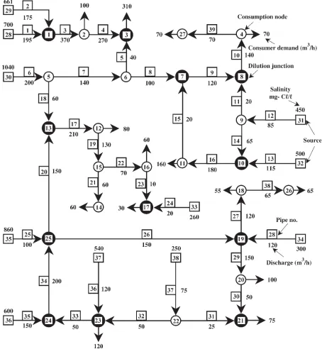
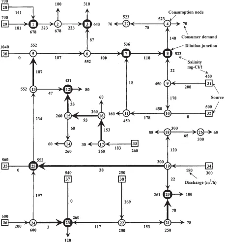
[image:11.569.54.508.57.549.2]The water supply system of the Central Arava region in southern Israel is an example of a regional multi-quality water distribution system. It supplies water both for irrigation and for domestic consumption. The layout of the network is presented in Figure 1. Note that pumps, boosters and control valves are not shown, since the hydraulics of the nework are not explicitly included in the model.
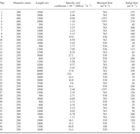
The initial flow discharges and directions in the network are shown in the figure, and characteristics of the 39 pipes are presented in Table I. The cost of water conveyance and specific cost coefficients were calculated from:
wip¼i jqiaj
1:852
and
i¼2:726103KeChwi1:852 d i
a
[image:12.569.61.514.72.504.2]4:87 ‘ia Table I. Data for pipes of the Central Arava network
Pipe Diameter (mm) Length (m) Specific cost Maximal flow Initial flow coefficient107(NIS m3h1) (m3h1) (m3h1)
1 300 2500 5.57 763 175
2 300 2000 4.46 763 195
3 400 1500 0.08 1357 370
4 400 2000 1.10 1357 270
5 300 500 1.11 763 40
6 300 1600 3.57 763 200
7 300 1000 2.23 763 140
8 300 2300 5.13 763 100
9 250 3500 19.0 530 120
10 300 4300 9.59 763 140
11 250 1000 5.42 530 20
12 250 500 2.71 530 85
13 250 1300 7.05 530 115
14 300 3700 8.25 763 65
15 250 5000 27.1 530 20
16 250 800 4.34 530 180
17 300 1200 5.58 763 210
18 300 4200 9.37 763 60
19 250 1000 5.42 530 130
20 300 8000 17.8 763 150
21 150 8000 522 190 60
22 250 2600 14.1 530 70
23 250 2000 10.8 530 10
24 300 2500 5.6 763 20
25 250 2600 14.1 530 100
26 400 4500 2.48 1357 150
27 300 1500 3.35 763 120
28 250 500 2.71 530 120
29 300 3000 6.69 763 150
30 250 500 2.71 530 50
31 250 800 4.34 530 25
32 300 2300 5.13 763 50
33 300 1800 4.02 763 50
34 300 3900 8.70 763 200
35 300 500 1.11 763 150
36 200 1000 16.1 339 120
37 250 2800 15.2 530 75
38 150 1300 84.8 190 65
wherewipis the conveyance cost in pipei,ithe specific cost coefficient for pipei,Kethe unit cost of energy, Chwi
the Hazen Williams coefficient for pipei(here Chw¼123) anddiaand‘iaare its diameter (mm) and length (m), respectively.
There are 37 nodes in the network, of which 11 are sources and 14 are consumers with various water quality requirements. The network is operated 4000 hours per year and cost per unit energy is 0.22 NIS kwh1. ($1ffi4:5 NIS at the time of this study. NIS¼new Israel shekel).
The water quality of the 11 source nodes is defined by three parameters, salinity, magnesium and sulphur. Specific costs and maximal discharges (m3h1) are summarized in Table II.
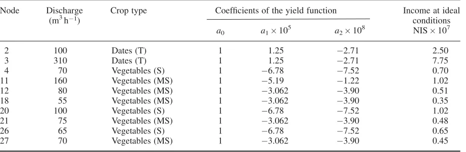
There are 10 agricultural consumers for which a quadratic yield function of the following form was defined with respect to salinity,y¼a0þa1cþa2c, whereyis the relative yield,cis the salinity in mg Cl l1, anda0,a1anda2 are constants as shown in Table III. Crop tolerance to salinity stress is categorized as tolerant (T), medium sensitive (MS) and sensitive (S). Expected income at ideal conditions of these crops is also given in Table III.
[image:13.569.54.512.70.233.2]There are four nodes requiring drinking water quality: 14, 16, 17 and 23. The maximum salinity at these nodes is 260 mg Cl l1, and the demand is 60 m3h-1 at nodes 14 and 16, 30 m3h-1at node 17 and 120 m3h-1 at node 23.
Table II. Data for sources
Node Specific cost Maximal discharge Water quality (mg Cl l1) (NIS m3) (m3h1)
Salinity Magnesium Sulphur
28 0.386 210 700 140 465
29 0.408 220 661 148 539
30 0.109 280 1040 110 860
31 0.638 200 450 148 401
32 0.554 200 500 148 401
33 0.735 200 260 72 400
34 0.713 180 300 73 465
35 0.256 150 860 110 670
36 0.458 200 600 155 690
37 0.535 150 540 142 720
38 0.723 300 250 65 354
Table III. Data for agricultural consumers’ nodes
Node Discharge Crop type Coefficients of the yield function Income at ideal
(m3h1) conditions
a0 a1105 a2108 NIS107
2 100 Dates (T) 1 1.25 2.71 2.50
3 310 Dates (T) 1 1.25 2.71 7.75
4 70 Vegetables (S) 1 6.78 7.52 0.70
11 160 Vegetables (MS) 1 5.19 1.22 1.02
12 80 Vegetables (MS) 1 3.062 3.90 0.51
18 55 Vegetables (MS) 1 3.062 3.90 0.35
20 100 Vegetables (S) 1 6.78 7.52 1.02
21 75 Vegetables (MS) 1 3.062 3.90 0.48
26 65 Vegetables (S) 1 6.78 7.52 0.65
27 70 Vegetables (MS) 1 3.062 3.90 0.45
[image:13.569.55.516.298.449.2]RESULTS AND DISCUSSION
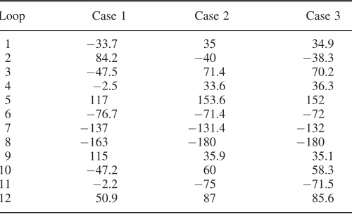
There are 12 loops and pseudo-loops in the network (see Figure 1). Two are real loops, (nodes 7, 8, 9, 10, 11) and (nodes 19, 20, 21, 22, 23, 24, 25), and the others are pseudo-loops, i.e. paths between the source nodes. The fundamental loops and pseudo-loops as determined by the solution process are presented in Table IV.
Three case studies were conducted:
1. Salinity is the only quality factor, no treatment plants;
2. Three water quality factors (salinity, sulphur, magnesium), no treatment plants; 3. Same as Case 2, but with treatment plants.
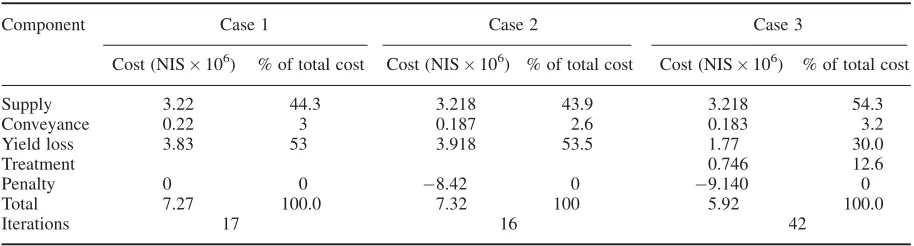
Values of the objective function, cost components, and the number of iterations required to obtain the optimal solutions are summarized in Table V.
[image:14.569.62.516.320.474.2]Examination of the results indicates that conveyance costs are very small. This is due to the large carrying capacity of the pipes. The discharge values at the optimal solution are much smaller than the design discharge values. Most of the cost (above 95%) in Cases 1 and 2 is the cost of water at the sources (supply cost) and the agricultural yield loss due to poor water quality. Treatment of irrigation water in Case 3 reduces the yield loss from about 3.83106NIS per year in Cases 1 and 2 to about 1.77106NIS per year in Case 3. The additional cost of treatment is about 0.746106NIS per year, yet the total cost of supply in Case 3 is lower (about 6106NIS per year, compared to about 7.3106NIS per year in Cases 1 and 2 without treatment), saving about 18% in
Table V. Values of objective function components for Cases 1, 2 and 3, in 106NIS per year
Component Case 1 Case 2 Case 3
Cost (NIS106) % of total cost Cost (NIS106) % of total cost Cost (NIS106) % of total cost
Supply 3.22 44.3 3.218 43.9 3.218 54.3
Conveyance 0.22 3 0.187 2.6 0.183 3.2
Yield loss 3.83 53 3.918 53.5 1.77 30.0
Treatment 0.746 12.6
Penalty 0 0 8.42 0 9.140 0
Total 7.27 100.0 7.32 100 5.92 100.0
[image:14.569.59.516.540.663.2]Iterations 17 16 42
Table IV. Loops and pseudo-loops in the network of Figure 1
Loop Type Between sources Pipes
1 b 28, 29 2 1
2 b 35, 30 6 18 20 25
3 b 35, 36 35 34 25
4 b 37, 36 35 33 36
5 b 38, 37 36 32 37
6 b 34, 38 37 31 30 29 28
7 b 35, 34 28 26 25
8 b 30, 33 24 23 22 19 17 18 6
9 b 31, 32 13 14 12
10 b 29, 30 6 7 5 4 3 2
11 a þ 16 15 14 11 9
12 a 30 29 26 31 32 33 34
the total cost. Optimal circular flows in the 12 loops and pseudo-loops for the 3 case studies are summarized in Table VI.
Case 1: Salinity as the only water quality parameter, no treatment plants
The optimal discharges in the pipes and salinity values at the nodes are shown in Figure 2. The following points should be noted:
discharges at the saline sources at nodes 30, 32, 35, 37 are zero;
flow directions have been reversed in pipes 18, 19, 22, 23, 26, 30 and 33 (compared to the initial directions as shown in Figure 1). These pipes are marked by a thick line in Figure 2.
These changes can be explained as follows: consumers 14 and 16 were initially supplied from the saline sources 30, 35 and 36, which have salinity values higher than the permitted values (see Figure 1). Water from sources 35 and 36 was diluted at node 25 in the initial flow distribution, and flow from node 25 was diluted by water from source 30. As a result, the salinity at consumers 14, 16 and 17 was higher than the permitted values. In the optimal solution, the flow directions in pipes 22 and 23 are reversed, allowing the flow of fresh water from source 33 so that the salinity limits at consumers 14, 16 and 17 are met.
The discharges from the saline water sources are reduced to zero in the optimal solution, as already mentioned, requiring additional amounts of water from the remaining sources in compensation. Salinity values at consumers 20 and 21 have been improved by dilution from sources 34 and 38. This has been obtained by a change in flow direction in pipe 30. Node 23 becomes a dilution junction between sources 36 and 38 such that the salinity limit at node 23 can be met. The solution uses some of the fresh water available at source 38 to improve the salinity at node 21 by about 50% and for dilution at node.
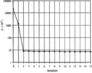
[image:15.569.157.407.70.222.2]The salinity at node 25 has been reduced to 551.8 mg Cl l1, from an initial value of 632.53 mg Cl l1. High quality water flows through pipe 20 to other parts of the network: 47 m3h1is diverted for dilution with water from source 33 to improve the salinity at consumer 12; and 187 m3h1to improve salinity in other parts of the network via pipe 18 whose flow direction was reversed. Part of this water flows from node 6 to improve salinity at consumer 3, and the remainder for reducing the salinity at consumers 4 and 27. The discharge in pipe 8 was not changed from its initial value, yet salinity dropped from 1040 to 551.8 mg Cl l1. Consumer 11 is supplied by water from source 31 only, so the original salinity of 450 mg Cl l1is not diluted by more saline water from source 32. Hence, the salinity limit for consumer 11 is met. This may be the reason why the discharge for pipe 13 is zero. The contribution from source 32 is therefore also zero to keep the salinity at node 11 at its limit. Change of objective function value with iteration of the solution procedure is shown in Figure 3. The optimal solution has essentially been reached after only three iterations, while in iterations 4–17 the improvement is only 3%.
Table VI. Values of optimal circular flows in m3h1, Cases 1, 2 and 3
Loop Case 1 Case 2 Case 3
1 33.7 35 34.9
2 84.2 40 38.3
3 47.5 71.4 70.2
4 2.5 33.6 36.3
5 117 153.6 152
6 76.7 71.4 72
7 137 131.4 132
8 163 180 180
9 115 35.9 35.1
10 47.2 60 58.3
11 2.2 75 71.5
Case 2: Three water quality parameters, no treatment plants
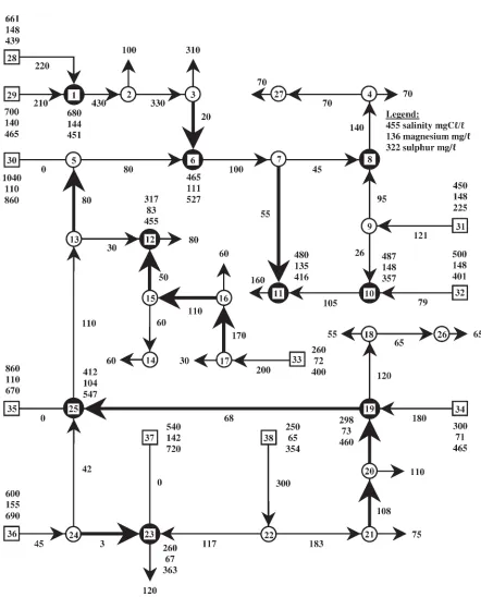
[image:16.569.59.517.57.548.2]Water quality is defined by three parameters: salinity, sulphur and magnesium (see Table II). Yield-loss functions for salinity at agricultural consumer nodes are the same as in Case 1 (with coefficients as given in Table III), while sulphur and magnesium constraints for irrigation water are expressed by upper limits only. Upper limits were also assumed for the three parameters at the high-quality domestic consumers. The limits were taken
from the Israel Water Quality Standard (1985) for drinking water. Standard potable water limits for salinity were used, and sulphur and magnesium upper limit values were included due to their high concentration at the sources. Additional bounds on sulphur and magnesium concentrations were set at consumers 4, 20 and 26 in which moderately sensitive vegetable crops are irrigated. The upper limits for the three parameters at the other consumer nodes are: salinity, 260 mg Cl l1 at consumers 14, 16, 17, 23; sulphur, 500 mg l1 at consumers 4 and 26, 437 mg l1at consumers 14, 16, 17, 23, and 400 mg l1at consumer 20; magnesium, 170 mg l1at consumers 4, 20, 26 and 150 mg l1at consumers 14, 16, 17 and 23.
[image:17.569.101.465.56.346.2]The solution was obtained after 16 iterations. Components of optimal objective functions are given in Table V. Composition of these components is very similar to that of Case 1 (salinity only) with a slight increase in yield losses and a 0.7% increase in the total cost due to the additional constraints on water quality. Values of circular flows in the loops and pseudo-loops are given in Table VI. Note the significant changes in loops 1, 2, 3, 4, 5, 9, 10, 11 and 12. Optimal distribution of discharges and quality parameters at the pipes and nodes of the network are shown in Figure 4. Flow distribution for Case 2 is significantly different from that of Case 1. The discharges from the saline sources 30, 35 and 37 are zero, while use of water from source 32 is essential since limits on sulphur and magnesium at source 4 require a discharge from source 31, and consequently from source 32, to meet the demand at consumer 11. This mix of supply water increases the salinity at consumer 11, leading to an increase in yield loss. Similarly, supply from source 38 is needed to meet the upper limit of magnesium at consumer 20. Consequently, flow directions have been reversed in pipe 29 and node 19 becomes a dilution junction between sources 34 and 38. Change in flow direction in pipe 26 causes node 25 to become a dilution junction for the high-quality water from sources 34, 35 and 36. This high-quality water is diverted to improve the water quality at consumers 4, 11 and 27, while meeting the water quality limits at consumers 20, 23 and 26 upstream along the flow direction. Salinity is improved at consumers 20, 21 and 26. The salinity at node 6 has dropped from 1040 to 412 mg Cl l1, magnesium concentration from 110.0 to 103.77 mg l1, and sulphur from 860 to 547 mg l1, all as a result of the change in flow direction in pipes 18 and 26. The change in flow direction in pipe 5 is required in order to decrease the sulphur
concentration at consumer 4 to a value below its upper limits value by dilution of water in pipe 7 with water from sources 28 and 29 where the sulphur concentration is low. The sulphur concentration in pipe 8 is still above the upper limits of consumer 4, however, so additional dilution is needed. Water with low sulphur content from source 31 is, therefore, diluted with water from pipes 8 and 9 at node 8 to reduce the sulphur concentration at consumer 4 to its upper limit. This additional water from source 31 forces the use of source 32 to reduce the yield loss at consumer 11. The flow direction in pipe 14 has been reversed and water of 500 mg Cl l1from source 32 is diluted by water of 456 mg Cl l1from node 6 via pipes 8 and 15. The number of junctions at which dilution occurs has been increased due to the increase in the number of water quality parameters from one (Case 1) to three (Case 2). In Case 1, dilution junctions are at nodes 1, 3, 8, 12, 20, 23 and 25, while in Case 2 they are at nodes 1, 6, 8, 10, 11, 12, 19, 23 and 25. This example demonstrates the need for simultaneous consideration of multiple water quality parameters.
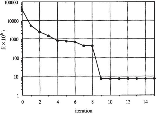
The convergence of the solution to its optimal value is shown in Figure 5. A significant change in the value of the objective function occurs at the eighth and ninth iterations. The solution method improves the objective function until the seventh iteration by increasing the number of active constraints. From the seventh iteration on, no improvement can be obtained by changing the composition of the active constraints, so a constraint is now omitted from the active set of constraints according to the values of the multipliers attached to the active constraints. Consequently, the direction of the projected gradient is changed, and new improvements in the value of the objective function are obtained after the eighth iteration. From the ninth to the sixteenth iterations, the improvement in the value of the objective function is minor. Termination criteria were met at the sixteenth iteration and the solution process stopped.
Case 3. Three water quality parameters with treatment plants
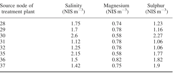
[image:19.569.118.449.410.650.2]The same three parameters as for Case 2 are used. In addition, treatment plants are attached to sources 28, 29, 30, 31, 32, 35, 36 and 37. The maximum allowable value of the removal ratio,r, at each plant was assumed to be 75%. Coefficients of the specific costs of treatment for the three water quality parameters at the treatment plants are given in Table VII.
Optimal discharge and concentration distributions in the network are shown in Figure 6.
The major change in this solution compared to the previous cases is in the flow direction in pipe 33. In Case 2, node 23 was a dilution junction for sources 36, 37 and 38 and the flow was from node 24 to 23 in pipe 33. In Case 3, the flow is from node 23 to 24 which become a dilution junction for sources 37, 38 and 36. Use of the saline sources 30 and 35 is not profitable even though they have treatment plants (see Table VIII). Water salinity at consumers 4 and 11 is lowered by operating the treatment plants at sources 31 and 32, and yield loss is reduced accordingly. The treatment at source 36 affects the quality at node 6 and consumers 4, 11 and 27. Treatment at sources 28 and 29 also reduces salinity levels at node 6 and consumers 2 and 3.
The solution was obtained after 42 iterations using the partial mixing step (PMS) method as described by Cohen
et al.(2000b, 2003). Cost components of the objective function are summarized in Table V. An additional cost component is included for treatment costs of 0.746106NIS per year, which are 12.6% of the total cost. Use of the treatment plants saves 19% in the total cost, most of which is due to a saving in yield loss from about 3.9106 NIS per year in Cases 1 and 2 without treatment plants, to about 1.7106NIS in Case 3, which includes treatment plants. There is no need to treat water for sulphur and magnesium, but the treatment plants for salinity have been operated at maximum removal ratio (r¼0.75) at sources 32 and 36 (Table VIII).
Optimal circular flows are given in Table VI. There is no significant difference in these values between Case 3 (with treatment plants) and Case 2 (without).
CONCLUSIONS
The model developed for optimal operation of multi-quality irrigation systems can be used for canal as well as for pipeline networks, since the hydraulics of the network are not explicitly included and are represented by the conveyance costs with wide bounds on maximum allowed discharge in each pipe/canal. A method was developed for the smooth representation of logical conditions, and dilution conditions and conveyance costs were expressed using this technique. Consequently, the derivatives of all functions in the model can be calculated and the operation problem becomes a regular nonlinear problem which can be solved using existing methods. However, inclusion of multiple water quality parameters and treatment plants presents further complications to the solution of the problem and a method has been developed and demonstrated that overcomes these problems. Treatment of water is considered here by reducing the concentration of conservative substances in the water, only excluding biological treatment, for example.
The model described demonstrates the following extensions of previous models:
[image:20.569.145.431.82.203.2]1. The network is undirected and water can flow any direction. Flow direction is included in the set of decision variables.
Table VII. Case 3. Coefficients of specific costs of treatment for the quality parameters
Source node of Salinity Magnesium Sulphur treatment plant (NIS m3) (NIS m3) (NIS m3)
28 1.75 0.74 1.23
29 1.7 0.78 1.16
30 2.6 0.58 2.27
31 1.12 0.78 1.06
32 1.25 0.78 1.06
35 2.15 0.58 1.77
36 1.5 0.82 1.82
37 1.42 0.75 1.9
2. The network includes treatment plants for conservative substances, and the solution includes the determination of their optimal removal ratios.
3. Cost of water at sources and conveyance costs within the network can be nonlinear.
4. Water quality can be defined by several conservative dependent and independent parameters. Any functional relationship between dependent and independent parameters can be accommodated.
5. Water quality demand at consumer nodes can be defined by upper limits, yield functions for agricultural crops, and/or benefit functions for urban consumers.
6. Application of the proposed method for regional networks with three water quality parameters and eight treatment plants has been demonstrated. However, the model has not yet been implemented, nor has it been used in practice. Many unexpected new problems may arise in course of realization of this mode, thus improvement and development are necessary.
ACKNOWLEDGEMENTS
Thanks are extended to Mr Selwyn Meyers MSc for his critical review and valuable comments regarding this paper, and to Mrs Ruth Adoni and Mr Arieh Aines for their help in the typing and graphics.
REFERENCES
Avriel M. 1976.Nonlinear Programming: Analysis and Methods. Prentice-Hall, Inc: New Jersey.
Cohen D. 1991. Optimal operation of multi-quality networks, DSc thesis, Faculty of Agricultural Engineering, Technion, Israel (in Hebrew), 400 pp.
Cohen D, Shamir U, Sinai G. 2000a. Optimal operation of multi-quality water supply systems–I. Introduction and the Q-C Model.Engineering Optimization32: 549–584.
Cohen D, Shamir U, Sinai G. 2000b. Optimal operation of multi-quality water supply systems–III. The Q-C-H Model. Engineering Optimization33: 1–35.
Cohen D, Shamir U, Sinai G. 2003. Comparison of models for optimal operation of multiquality water supply networks.Engineering Optimization35(6): 579–605.
Feinerman E, Yaron D. 1983. Economics of irrigation water mixing within a farm framework.Water Resources Research19(2): 337–345. Jensen PK, Matsuno Y, van der Hoek W, Cairncross S. 2001. Limitations of irrigation water quality guidelines from a multiple use perspective.
Irrigation and Drainage Systems15: 117–128.
Maas EV, Hoffman GJ. 1977. Crop salt tolerance–current assessment.Journal of Irrigation and Drainage ASCE103: 115–134.
Mehrez A, Percia C, Oron G. 1992. Optimal operation of multi-sources and multiquality regional water systems.Water Resources Research 28(5): 1199–1206.
Meiri A, Shalhevet J, Stolzy LH, Sinai G, Steinhardt R. 1986. Managing multi-sources irrigation water of different salinities for optimum crop production. Final report to BARD (USA–Israel Binational Agricultural Research Fund) No. I-402–81 Volcani Center, POB 6, Bet Dagan Israel.
Oron G. 1987. Marginal water application in arid zones.Geographical Journal15(3): 259–266.
Ostfeld A, Shamir U. 1993. Optimal operation of multiquality networks–I: Steady-state conditions.Journal of Water Resources Planning and Management ASCE119(6): 645–662.
Percia C, Oron G, Mehrez A. 1997. Optimal operation of regional system with diverse water quality sources.Journal of Water Resources Planning and Management ASCE123(2): 105–115.
Pessen D, Reike M, Sinai G. 1986. Design and simulation of water mixing junctions in irrigation systems.International Journal of Modelling and Simulation6(1): 32–38.
[image:22.569.61.517.71.112.2]Pessen D, Sinai G, Fasol KH, Reike M. 1989. Design of dilution junctions for water quality control.Journal of Water Resources Planning and Management ASCE115(6): 829–845.
Table VIII. Case 3. Optimal removal ratio for salinity treatment plants
Source node 28 29 30 31 32 35 36 37
Schwartz J, Meidad N, Shamir U. 1985. Water quality management in regional systems. InProceedings of Jerusalem Symposium on Scientific Basis for Water Resources Management, IAHS Pub. 153; 341–349.
Shah M, Sinai G. 1985. Salinity control in multi-quality irrigation networks–Kibbutz Hamadia feasibility study. Agricultural Water Management10: 235–252.
Shah M, Sinai G. 1988. A steady state model for dilution in water networks.Journal of Hydraulic Engineering, ASCE114(2): 192–206. Shamir U. 1983. Management of regional multiple quality water supply systems. InProceedings of Hamburg Symposium on Scientific Process
Applied to Planning, Design and Management of Water Resources Systems, IAHS Pub. 147; 407–421.
Sinai G, Koch E, Farbman M. 1985. Dilution of brackish water in irrigation networks–an analytic approach,Irrigation Science6: 191–200. Sinai G, Shina G, Kitai E, Shah M. 1987. Physical and computer models of multi-quality networks.Journal of Water Resources Planning and
Management ASCE113(6): 745–760.