Ann. Geophys., 31, 2157–2162, 2013 www.ann-geophys.net/31/2157/2013/ doi:10.5194/angeo-31-2157-2013
© Author(s) 2013. CC Attribution 3.0 License.
Annales
Geophysicae
Open Access
Equatorial spread F studies using SAMI3 with two-dimensional and
three-dimensional electrostatics
H. C. Aveiro1and J. D. Huba2
1National Research Council Postdoctoral Fellow at the Naval Research Laboratory, Washington, DC, USA 2Plasma Physics Division, Naval Research Laboratory, Washington, DC, USA
Correspondence to: H. C. Aveiro ([email protected])
Received: 28 June 2013 – Accepted: 15 November 2013 – Published: 5 December 2013
Abstract. This letter presents a study of equatorial F re-gion irregularities using the NRL SAMI3/ESF model, com-paring results using a two-dimensional (2-D) and a three-dimensional (3-D) electrostatic potential solution. For the 3-D potential solution, two cases are considered for paral-lel plasma transport: (1) transport based on the paralparal-lel am-bipolar field, and (2) transport based on the parallel electric field. The results show that the growth rate of the generalized Rayleigh–Taylor instability is not affected by the choice of the potential solution. However, differences are observed in the structures of the irregularities between the 2-D and 3-D solutions. Additionally, the plasma velocity along the geo-magnetic field computed using the full 3-D solution shows complex structures that are not captured by the simplified model. This points out that only the full 3-D model is able to fully capture the complex physics of the equatorial F region.
Keywords. Ionosphere (Equatorial ionosphere; Modeling and forecasting; Plasma waves and instabilities)
1 Introduction
Equatorial spread F (ESF) refers collectively to a family of plasma density irregularities that form in the equatorial F re-gion ionosphere after sunset. The phenomenon has been ex-tensively studied with the support of coherent scatter radars, ionosondes, airglow imagers, ground-based scintillation re-ceivers, and instruments onboard rockets and satellites (see details in Woodman, 2009).
Topside ESF irregularities are driven by the generalized Rayleigh–Taylor instability near and above the F peak, and the plasma instability mechanism seems to be well
under-stood. However, the first stages of ESF irregularity devel-opment, namely bottom-type and bottomside irregularities, and the plasma instabilities behind those two processes, have not been fully explained to date. Some of the mechanisms that have been proposed to explain the triggering of plasma waves are vertical shear in the horizontal plasma flow (Hy-sell and Kudeki, 2004), gravity waves (Huang and Kelley, 1996), and large-scale wave structure in the bottomside of the ionosphere (Tsunoda, 2005).
Numerical simulations have been used as a tool for the un-derstanding of ESF. Three-dimensional models incorporating equipotential field lines (two-dimensional ionospheric poten-tial solvers) have been extensively used (as, e.g., Huba et al., 2008 and Retterer, 2010). Two-dimensional ionospheric po-tential solvers use the fact that the plasma conductivity com-ponent parallel to the magnetic field is several orders of mag-nitude higher than the conductivity in the perpendicular di-rection, such that the magnetic field lines are assumed to be equipotential. This removes the dependence of the iono-spheric potential in the dimension along the magnetic field, reducing the problem from 3-D to 2-D. Recent studies have shown that only 3-D models are able to capture the full nature of ESF (see, e.g., Aveiro and Hysell, 2010). Using both a 2-D and a 3-D ionospheric model, Aveiro and Hy-sell (2012) showed that the former is not able to simulate the initial stages of ESF and that only the 3-D model could simulate the 3 stages of ESF: bottom-type, bottomside, and topside. Their model was simplified in the sense that it only accounted for three ions: O+, O
2158 H. C. Aveiro and J. D. Huba: ESF modeling using SAMI3
−20 0 20 40 60 80 100
Vφ[m/s] 100
200 300 400 500 600
Altitude
[km]
U V2D
V3DA
V3DF
2 3 4 5 6 7
log10ne[cm−3]
100 200 300 400 500 600
Altitude
[km]
−10 −5 0 5 10
0.0 0.5 1.0 1.5 2.0 2.5 3.0
δ
Φ[
V
]
−10 −5 0 5 10
102
103
104
105
106
107
ne
[cm
−
3]
−10 −5 0 5 10
Magnetic Latitude [◦] 100
200 300 400 500
Altitude
[km]
Figure 1.
Initial conditions for the ESF model run (
t
0= 19:00 LT) at
φ
=0. (Left)
Vertical cut: (top) plasma density and (bottom) zonal plasma drifts for (blue) 2D, (green)
3D-A, and (red) 3D-F electrostatic models. (Dashed) Local zonal wind speeds are also
depicted for reference. (Right) Cut through the meridional plane at 440 km apex altitude
: (top) electrostatic potential, (middle) plasma density, and (bottom) equivalent altitude.
D R A F T
April 26, 2013, 1:58pm
D R A F T
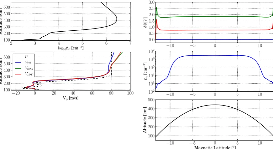
Fig. 1. Initial conditions for the ESF model run (t0= 19:00 LT) atφ= 0. (Left) Vertical cut: (top) plasma density and (bottom) zonal plasma drifts for (blue) 2-D, (green) 3-D-A, and (red) 3-D-F electrostatic models. (Dashed) Local zonal wind speeds are also depicted for refer-ence. (Right) Cut through the meridional plane at 440 km apex altitude: (top) electrostatic potential, (middle) plasma density, and (bottom) equivalent altitude.
simulate the evolution of a topside ESF plasma irregularity using SAMI3/ESF with three different methods for the solu-tion of the electrostatic potential: (1) 2-D potential (equipo-tential flux tubes), (2) 3-D po(equipo-tential with parallel transport using the ambipolar electric field associated with the parallel electron pressure (3-D-A), and (3) 3-D potential with par-allel transport using the parpar-allel electric field (3-D-F). The main goal is to evaluate how well the three approaches per-form in terms of the physics captured and the complexity of the model for the simulation of plasma irregularities in ESF.
2 SAMI3/ESF model
The model was constructed using magnetic dipole coordi-nates (p, q, φ), where the tilt is matched to the magnetic declination in the longitude of interest. In our terminology,
prepresents the McIlwain parameter (L),q is the magnetic co-latitude, andφis the longitude. The background current density including zonal wind forcing, plasma pressure, and gravity-driven currents is given as:
J0= ˆ6·(U×B)+ ˆD· ∇n+ ˆ0·g, (1) where the terms on the right-hand side (RHS) represent the ohmic, diffusion, and gravity-driven currents, respectively. The terms6ˆ,Dˆ, and0ˆ represent the conductivity, diffusion, and gravity tensors, respectively (see, e.g., Shume et al., 2005 for an explicit definition of those terms). The variablesUand
Bare the neutral wind speed and magnetic field, respectively. Perpendicular diffusion currents are neglected in the current version of the model, since their contribution is very small compared to the other two terms on the RHS.
The computation of the electrostatic potential is based on the solenoidal current density (∇ ·J=0) and can be written as
∇ ·h6ˆ · ∇8i= ∇ ·J0, (2)
where J=J0− ˆ6· ∇8. In the 3-D model, Eq. (2) is solved directly in all 3 dimensions (p, q, φ).
In the 2-D model, the approach uses the fact that parallel conductivities are much larger than any of the perpendicular conductivities (Hall or Pedersen). Equation (2) is integrated along the parallel direction and the following condition is ob-tained:
Z ∂Jk
∂s ds=0, (3)
where the RHS is null, since parallel currents vanish at the bottom boundary of the ionosphere. This approach also indi-cates that there are no variations in the electrostatic potential alongB, i.e., the field lines are equipotential.
[image:2.595.79.515.63.301.2]H. C. Aveiro and J. D. Huba: ESF modeling using SAMI3 2159
−200 −100 0 100 200
200 300 400 500 600 Apex Alt. [km] ne2D
−15 −10 −5 0 5 10 15
200 300 400 500 600
Vk2D
−200 −100 0 100 200
200 300 400 500 600 Apex Alt. [km]
ne3D−A
−15 −10 −5 0 5 10 15
200 300 400 500 600
Vk3D−A
−200 −100 0 100 200
Ground horizontal distance (km)
200 300 400 500 600 Apex Alt. [km]
ne3D−F
3.2 3.6 4.0 4.4 4.8 5.2 5.6 6.0 6.4 log10ne[cm−3]
−15 −10 −5 0 5 10 15
Magnetic Latitude [◦] 200
300 400 500 600
Vk3D−F
−5 −4 −3 −2 −1 0 1 2 3 4 5
[image:3.595.74.522.65.351.2]Vk[km/s]
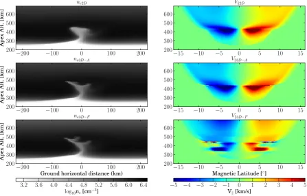
Fig. 2. Plasma conditions at the end of the simulation (t∼21:00 LT): (left) plasma densities in a cut through the equatorial plane and (right) O+ion parallel velocities in a cut through the meridional plane. From top to bottom, the solutions using the 2-D, 3-D-A, and 3-D-F models, respectively.
simplifies to ∂
∂p6Pp+ ∂ ∂φ6H
∂8
∂p +
− ∂
∂p6H+ ∂ ∂φ6Pφ
∂8
∂φ
=∂j0p
∂p + ∂j0φ
∂φ , (4)
where
6Pp=
Z
σP
hp hφ
hqdq, 6Pφ=
Z
σP
hφ hp
hqdq,
6H= Z
σHhqdq (5)
and
j0p=
Z
J0· ˆphφhqdq, j0φ=
Z
J0· ˆφhphqdq. (6)
The termspˆ andφˆ are unit vectors, andσPandσHare the Pedersen and Hall conductivities, respectively. Thehi
coef-ficients are the scale factors that arise from the spherical to magnetic dipole coordinate system transformation (see, e.g., Huba et al., 2000), where the indexirefers to the direction and8represents the electrostatic potential.
Both Eqs. (4) and (2) are solved using the Bi-Conjugate Gradient Stabilized (BiCGStab) method using the SPARSKIT sparse matrix solver numerical library (Saad,
1990). The computational complexity increases with the ma-trix size and is O(N) for sparse mama-trix solvers. For in-stance, for a 3-D spatial grid nφ=96,np=130, andnq=130
points, the 2-D potential matrix would be 12 480×12 480 and 1 622 400×1 622 400 for the full 3-D potential case.
Alongside the electrostatic potential, equations for the ion momentum and continuity are solved (see Huba et al., 2000 for a full description). The ion momentum equation in the parallel direction can be written as
DVik ∂t = −
1
nimi
∇kPi+
e mi
Ek+gk
−νin(Vik−Uk)−
X
j
νij(Vik−Vjk), (7)
where Vik, Pi, ni, and mi represent the parallel velocity,
plasma pressure, density, and mass for the i ion species, respectively. The terms νin and νij are the collisions
be-tween the i ion species with the neutrals and the j ion species, respectively. The electric field component in the par-allel direction comes from the electrostatic potential (Ek= −∇k8) in the 3-D-F model, and it is ambipolar (Ek= −∇kPe/ne) in both the 2-D and 3-D-A models. Finally,
−
10
−
5
0
5
10
10
210
310
410
510
610
7ne
[cm
−
3] 2D
3DA 3DF
−
10
−
5
0
5
10
−
4
−
2
0
2
4
Vk
[km/s]
−
10
−
5
0
5
10
Magnetic Latitude [◦]
100
200
300
400
500
Altitude
[km]
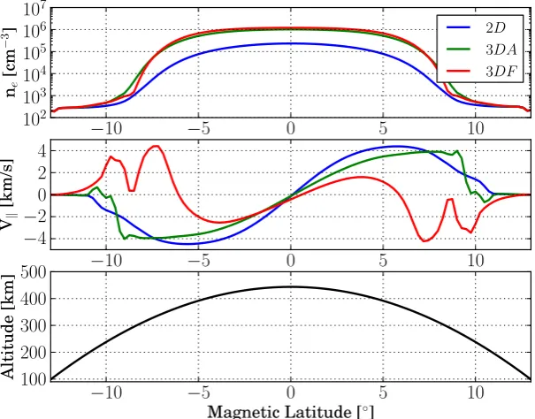
Fig. 3. (Top) Plasma densities and (middle) O+ion parallel velocities along the flux tube that intercepts the top of the plasma irregularity (∼440 km apex altitude) for the (blue) 2-D, (green) 3-D-A, and (red) 3-D-F models. The bottom panel depicts the equivalent altitude (in km) at a given point.
A major simplification to the momentum equation in the perpendicular direction is made through the assumption that the main forcing is due toE×Bdrifts. This condition will be relaxed in the next version of the model. The transport is per-formed using a Monotone Upwind Scheme for Conservation Laws (MUSCL) with the Sweby flux limiter (see, e.g., Trac and Pen, 2003) using a second-order Runge–Kutta method for the integration of the continuity equation in the perpen-dicular direction. The original SAMI3 model uses the donor cell method, which is only first-order accurate.
3 Model setup and results
The zonal boundaries of the model are periodic and the grid size isnφ= 96,np= 130, andnq=130 points. The grid
is ±2◦ wide in longitude and spans between 90–690 km apex altitudes (L= 1.014–1.108). The simulation runs start att0= 19:00 LT and the initial plasma conditions (densities and velocities) are obtained from a 36 h SAMI2 model run (Huba et al., 2000). A Gaussian perturbation is imposed on the plasma density at the bottomside of the F region.
Figure 1 depicts the initial conditions for the simulation runs atφ=0. The left panels show diagnostics in the ver-tical direction at the magnetic equator. Zonal plasma drifts for all three models are similar below the F peak. The zonal shear node is located at∼240 km, where the density gradient of the F region bottomside is very steep. At alti-tudes above∼400 km the 2-D and the 3-D solutions differ,
and the 2-D solution reflects the local zonal wind speeds (∼80 m s−1). Zonal plasma drifts for the 3-D models were slightly faster (∼90 m s−1), but were still slower than the maximum zonal wind speeds in the same flux tube (although not shown here, the magnitude of the zonal wind velocity reaches∼120 m s−1 off-equator for these runs). This indi-cates that comparisons between local plasma drifts and neu-tral wind observations may be correlated, but differences of the order of 10 % might be expected (based on these sim-ulation runs). Note that the higher in altitude the simula-tion goes, the larger the difference between the local neutral and plasma zonal velocities gets due to large off-equatorial Pedersen conductivities.
[image:4.595.147.450.65.302.2]H. C. Aveiro and J. D. Huba: ESF modeling using SAMI3 2161
model assumes equipotential field lines such that the electro-static potential does not vary along the flux tube.
Figure 2 shows the results at the end of the simulation (t∼21:00 LT): (left) plasma densities in a cut through the equatorial plane and (right) O+ ion parallel velocities in a cut through the meridional plane. From top to bottom, the solutions using the 2-D, 3-D with ambipolar electric field (3-D-A), and full 3-D model (3-D-F) runs, respectively. At 21:00 LT the instability was at the same stage of develop-ment in all model runs and the plasma irregularities had all crossed through the F peak (located at∼380 km altitude). The plasma irregularity in the 2-D model was wider in longi-tude, indicating a zonal ballooning expansion. This indicates that the 2-D solution for the potential was smoother than in the 3-D models, and consequently the zonal plasma drifts were pointing outward from the center of the plasma irregu-larity over a larger zonal span. The opposite was observed in the 3-D models, where the more complex structure of the per-pendicular electric fields and drifts was preserved, leading to short-scale forms and bifurcation (although not shown here, the plasma irregularities also bifurcated in the 2-D run, but at a later time step). The plasma density results for the 3-D models (3-D-A and 3-D-F) showed small differences above the F peak, but most of their structures remained similar. E-folding growth times estimated from the maximum vertical velocity time series were∼14 min for all of the model runs, indicating that the generalized Rayleigh–Taylor instability is not affected by the choice of the potential solution.
Remarkable differences between the three models are seen in the O+ion parallel velocities in a cut through the merid-ional plane at the center of the plasma irregularity. Both 2-D and 3-D-A models presented a similar poleward plasma flow structure with steep gradients near the top of the plasma irregularity. The full model solution (3-D-F) showed addi-tional structures in the parallel velocity that were not detected in the other two runs. Figure 3 shows a slice of the plasma densities and O+ion parallel velocities along the flux tube that intercepts the top of the plasma irregularity (at∼440 km apex altitude). O+ion parallel velocities showed regions with enhanced equatorward flow at both the low latitude F valley and bottomside. Note that the simplified versions of the elec-trostatics model (2-D and 3-D-A) were not able to capture those features. The redistribution of the plasma density in the parallel direction for the 2-D model run was smoother than in the 3-D models, indicating enhanced parallel diffu-sivity. This seems to be caused by the absence of gradients in the perpendicular forcing along the magnetic field (∇kJ0⊥),
since the 3-D-A model did not include any background cur-rent in the parallel direction (J0k=0), but was less diffusive
than the 2-D model.
4 Discussions and conclusions
This letter presented a comparative study of the evolution of equatorial F region irregularities using a two-dimensional and a three-dimensional electrostatic potential solution in the NRL SAMI3/ESF model. For the 3-D potential solu-tion, two cases are considered for parallel plasma trans-port: (1) transport based on the parallel electric field, and (2) transport based on the parallel ambipolar field. The results showed that the growth rate of plasma irregularities due to the Rayleigh–Taylor instability was unaffected by the choice of the ionospheric electrostatic potential approach. This was already expected, since the F region dynamo dominates dur-ing the nighttime, when the low latitude E region plasma conductivities are small. The growth rate of the generalized Rayleigh–Taylor instability is larger in collisionless regions and where the zonal background electric field is stronger, i.e.,
∼(g/νin+E/B)n0/n, and such parameters were not largely
affected by the choice of the electrostatic potential approach. However, the parallel flow was different. The typical pole-ward flow was observed when the potential solution did not include any forcing along the magnetic field, but a more structured flow with diverging and converging parallel flows was observed when the potential was fully solved in 3-D. Other differences included the lack of both fine structure and bifurcation in the 2-D solution when comparing the models at the same stage of evolution, which indicates that the 2-D solution for the ionospheric electrostatic potential does not fully describe the plasma flow structure of the ionosphere during equatorial spread F events, and therefore computing the full 3-D solution is necessary in order to capture the com-plex physics of the equatorial F region.
Acknowledgements. This research was performed while one of the
authors (H.C.A.) held a National Research Council Research Asso-ciateship Award at the US Naval Research Laboratory. The research of J.D.H. was supported by NRL Base Funds.
Topical Editor J. Retterer thanks M. Jonathan and I. S. Batista for their help in evaluating this paper.
References
Aveiro, H. C., and Hysell, D. L.: Three-dimensional numer-ical simulation of equatorial F-region plasma irregularities with bottomside shear flow, J. Geophys. Res., 115, A11321, doi:10.1029/2010JA015602, 2010.
Aveiro, H. C., and Hysell, D. L.: Implications of the equipotential field line approximation for equatorial spread F analysis, Geo-phys. Res. Lett., 39, L11106, doi:10.1029/2012GL051971, 2012. Huang, C.-S., and Kelley, M. C.: Nonlinear evolution of equatorial spread F: 4. Gravity waves, velocity shear, and day-to-day vari-ability, J. Geophys. Res., 101, 24521–24532, 1996.
Huba, J. D., Joyce,G., and Krall, J.: Three-dimensional equa-torial spread F modeling, Geophys. Res. Lett., 35, L10102, doi:10.1029/2008GL033509, 2008.
Hysell, D. L. and Kudeki, E.: Collisional shear instability in the eqautorial F region ionosphere, J. Geophys. Res., 109, A11301, doi:10.1029/2004JA010636, 2004.
Retterer, J. M.: Forecasting low-latitude radio scintillation with 3-D ionospheric plume models: 1. Plume model, J. Geophys. Res., 115, A03306, doi:10.1029/2008JA013839, 2010.
Saad, Y., SPARSKIT: A basic tool kit for sparse matrix computa-tions, Tech. Rep. RIACS-90-20, Research Institute for Advanced Computer Science, NASA Ames Research Center, 1990.
Shume, E. B., Hysell, D. L., and Chau, J. L.: Zonal wind veloc-ity profiles in the equatorial electrojet derived from phase ve-locities of type II radar echoes, J. Geophys. Res., 110, A12308, doi:10.1029/2005JA011210, 2005.
Trac, H. and Pen, U. L.: A primer on Eulerian computational fluid dynamics for astrophysicists, Astrophysics, 115, 303–321, 2003. Tsunoda, R. T.: On the enigma of day-to-day variability in equato- rial spread F, Geophys. Res. Lett., 32, L08103, doi:10.1029/2005GL022512, 2005.