Intelligent drought tracking for its use in
Machine Learning: implementation and first
results
Vitali Diaz
1,2*, Gerald A. Corzo Perez
2, Henny A.J. Van Lanen
3and Dimitri
Solomatine
1,21 IHE Delft Institute for Water Education, Delft, 2601 DA, the Netherlands
2 Delft University of Technology, Delft, the Netherlands
3 Hydrology and Quantitative Water Management Group, Wageningen University, Wageningen,
Droevendaalsesteeg 3a, 6708 PB, the Netherlands
Abstract
Due to the underlying characteristics of drought, monitoring of its spatio-temporal development is difficult. Last decades, drought monitoring have been increasingly developed, however, including its spatio-temporal dynamics is still a challenge. This study proposes a method to monitor drought by tracking its spatial extent. A methodology to build drought trajectories is introduced, which is put in the framework of machine learning (ML) for drought prediction. Steps for trajectories calculation are (1) spatial areas computation, (2) centroids localization, and (3) centroids linkage. The spatio-temporal analysis performed here follows the Contiguous Drought Area (CDA) analysis. The methodology is illustrated using grid data from the Standardized Precipitation Evaporation Index (SPEI) Global Drought Monitor over India (1901-2013), as an example. Results show regions where drought with considerable coverage tend to occur, and suggest possible concurrent routes. Tracks of six of the most severe reported droughts were analysed. In all of them, areas overlap considerably over time, which suggest that drought remains in the same region for a period of time. Years with the largest drought areas were 2000 and 2002, which coincide with documented information presented. Further research is under development to setup the ML model to predict the track of drought.
1
Introduction
Drought is costly and its damages are observed around the globe (Below et al., 2007; Mishra and Singh, 2010; Sheffield and Wood, 2011; Tallaksen and Van Lanen, 2004; Wilhite, 2000). It is a regional
Engineering Volume 3, 2018, Pages 601–606
phenomenon that covers, sometimes, large territorial extensions (World Meteorological Organisation (WMO), 2006). It is argued that a greater understanding of how drought develops, incl. where it moves over time, that is spatio-temporal dynamics, may help to better monitor drought.
Usually, drought monitoring is conducted through snapshots of the temporal development of a drought indicator (DI). This DI transforms the hydro-meteorological record into values related to drought anomalies (Mishra and Singh, 2010). When DI is computed in a spatially distributed way, the study region is schematized as a grid and in each cell, the DI is calculated. Through setting a DI threshold, it is possible to classify a cell whether it is in a drought event or not. This condition of non-drought/drought can be expressed in a binary way, i.e. using 0s and 1s (Corzo Perez et al., 2011). Neighbouring cells showing the same drought condition can be aggregated into regions (areas) by applying a clustering technique. Currently, available drought monitors provide information about the spatial extent of droughts (i.e. snapshots) but still the tracking of these drought areas is lacking.
This study aims to explain the main principles of a new method for drought monitoring by tracking its spatial extent. The output will be used in ML models, in which inputs are linked to outputs with a group of methods that learn/forget, and interact with each other (Solomatine and Siek, 2006). In this paper, the description and preliminary results of the proposed methodology to calculate drought trajectories is presented. In the next section, description of the methodology and its implementation are shown. The spatio-temporal Contiguous Drought Area (CDA) analysis is described as well. As India is a country highly prone to drought, it was used in this pilot as an example. After, the results of the computation of drought trajectories for India from 1901 to 2013, is presented. We conclude with a discussion and main findings.
2
Material and methods
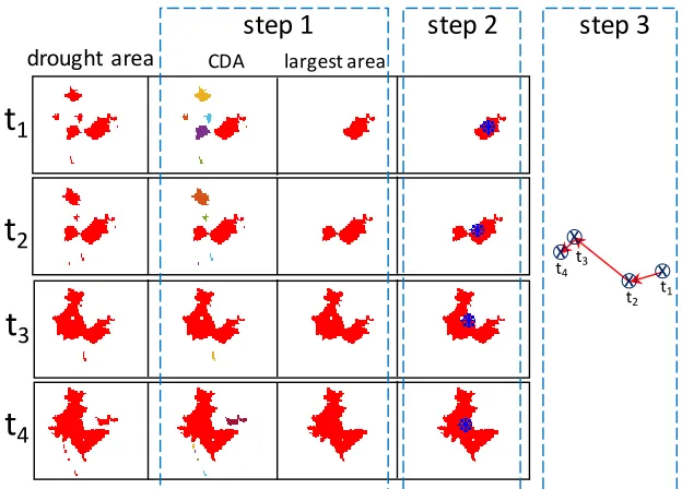
Three main steps were followed to determine the drought tracks: (1) calculation of the spatial drought events (referred to here also as areas, or clusters); (2) localization of spatial drought events centroids; (3) tracking droughts through the estimation of the trajectory of centroids (Figure 1). The spatial drought areas are identified by means of the Contiguous Drought Area (CDA) analysis (Corzo Perez et al., 2011) on a monthly basis. A CDA is composed of neighbouring regions (cells) in drought. Following the CDA methodology, at each time step, the CDAs are computed. After this, the major (largest) drought areas and their centroids are found. Drought tracks are built by following the centroids in time. A threshold of Euclidean distance between consecutive drought areas is applied to separate/join the sequence.
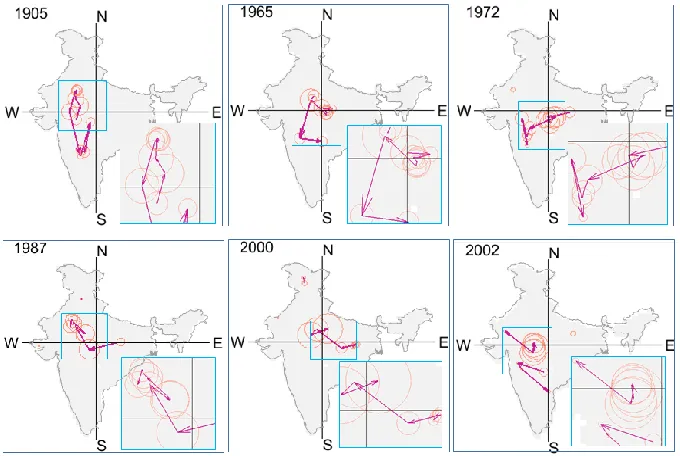
Drought tracks were analysed in two parts: (1) the patterns of all trajectories of largest drought areas for the whole period (1901-2013), and (2) the patterns in the worst reported droughts. To select the years with the most severe drought registered, two sources were consulted and analysed to provide relevant information. According to data (1900-2009) from the Centre for Research on the Epidemiology of Disasters (CRED) (Below et al., 2007) and the Monthly Weather Review (Bhalme and Mooley, 1980), India was impacted severely by droughts in 1900, 1905, 1942, 1964/1965, 1972, 1979, 1982, 1987, 1993, 1996, 2000, 2002, and 2009. Some of these years showed droughts during the monsoon rainfall, which is the Indian rainy season (Bhalme and Mooley, 1980). The years with the worst drought throughout the period were 1987 and 2002. The years selected for the second part of the analysis were 1905, 1965, 1972, 1987, 2000, and 2002.
3
Results and discussion
The results are presented in two parts. First, the patterns of all tracks of largest drought areas along the period 1901-2013 were examined. Second, droughts in the worst 6 years in drought (Section 2). For both parts, SPEI-6 was used to detect drought and CDA to compute its spatial extent. An estimation of drought trajectories was done by tracking the centroid of drought extents.
Drought patterns were estimated for the period 1901 to 2013 (Figure 2). Centroids of the largest drought areas are presented in Figure 2 (top). The spatial drought extent is shown schematically with symbols that indicate four intervals of percentage of drought area with respect to the country. The origin of the axes is placed in the centre of the country. It is observed that the spatial distribution of the centroids is almost uniformly distributed over India. However, a higher density of the areas with considerable extent can be seen in central India. Drought tracks are shown in Figure 2 (bottom). Three drought paths were detected when observing the historical drought tracks. These are (1) N to S, (2) E to S, and (3) E to W.
x
x
x
x
drought area
step 1
step 2 step 3
t
1
t
2
t
3
t
4
t1
t2
t3
t4
CDA largest area
Figure 2: Centroids of the largest drought areas identified on a monthly basis (top). Spatial drought extent schematized by four symbols pointing out the percentage of drought area. Drought tracks identified on a monthly basis for the analysis period (bottom). The origin of the axes is placed in the centre of the country
Drought tracks for 1905, 1965, 1972, 1987, 2000, and 2002 are presented in Figure 3. In all cases, it is observed that drought areas overlap considerably, which suggests that the spatial extent after reaching a considerable size, it remains in the same region. The presence of large drought areas in the same region over time may explain the severity of drought events in these years. There is no predominant route followed by droughts in these years, but similar tracks were identified in 1905 and 1965, as well as 1987 and 2000. The western part of India seems to be the region where the centres of the worst drought events were located, for example, see 1905, 1987 and 2002 in Figure 3. For the most extreme drought events (1987, 2002) a certain pattern was detected: they started from N to S, then changed their trajectory into the opposite direction. In terms of spatial extent, 2000 and 2002 events were the largest.
W
N
S
E
W
N
S
E
W
N
S
E
W
N
S
Figure 3: Drought trajectories (red arrows) of selected years with the most severe droughts. Spatial drought extent is schematized by a circle where its centre corresponds to the respective centroid. Insets show zoomed-in views. For the sake of clarity, a reduction factor was used to show the circles
4
Conclusions and future research
The presented methodology allowed comparing historical droughts and analysing their spatio-temporal dynamics. Some preliminary conclusions for India can be drawn from these first results.
From the historical overview from 1901 to 2013:
Spatial distribution of the centroids of the largest droughts areas is almost uniform across the country.
Density of the spatial distribution of drought events with considerable drought coverage is higher in central India.
Preferred routes by droughts were detected when observing the historical drought tracks.
Regarding the worst years in drought: 1905, 1965, 1972, 1987, 2000, and 2002:
For these years, it is observed that drought areas overlap considerably, which suggests that drought remained in the same region (i.e., high spatial persistence).
There is no predominant route followed by droughts in these years.
The western part of India seems to be the part where the centres of the worst drought events were located.
For the most extreme drought events (1987, 2002) a certain pattern was detected: they started from N to S, then changed their trajectory into the opposite direction.
The analysis presented here is being also validated through a leave one out procedure, evaluating the reliability of the data and the determination of the level of accuracy in the proposed method. With the drought tracks built, further research is under development to set up the model based on ML. The final outcome of this research will be a model that predicts the drought track. The development of this model and other aspects of the study can be consulted at www.researchgate.net/project/STAND-Spatio-Temporal-ANalysis-of-Drought.
Acknowledgements
Vitali Diaz thanks the Mexican National Council for Science and Technology (CONACYT) for the study grand 217776/382365. HvL is supported by the H2020 ANYWHERE project (Grant Agreement No. 700099).
References
Beguería, S., Vicente-Serrano, S.M., Reig, F., and Latorre, B. (2014). Standardized precipitation evapotranspiration index (SPEI) revisited: parameter fitting, evapotranspiration models, tools, datasets and drought monitoring. International Journal of Climatology, 34(10), 3001–3023. doi:http://doi.org/10.1002/joc.3887
Below, R., Grover-Kopec, E., and Dilley, M. (2007). Documenting drought-related disasters: a global reassessment. The Journal of Environment and Development, 16(3), 328–344. doi:http://doi.org/10.1177/1070496507306222
Bhalme, H.N., and Mooley, D. (1980). Large-scale droughts/floods and monsoon circulation. Monthly Weather Review, 108(8), 1197–1211. doi:http://doi.org/10.1175/1520-0493(1980)108<1197:LSDAMC>2.0.CO;2
Corzo Perez, G.A., Van Huijgevoort, M.H.J., Voß, F., and Van Lanen, H.A.J. (2011). On the spatio-temporal analysis of hydrological droughts from global. Hydrology and Earth System Sciences, 15(9), 2963–2978. doi:http://doi.org/10.5194/hess-15-2963-2011
Mckee, T.B., Doesken, N.J., and Kleist, J. (1993). The relationship of drought frequency and duration to time scales. AMS 8th Conference on Applied Climatology, January, pp. 179–184. doi:http://doi.org/citeulike-article-id:10490403
Mishra, A.K., and Singh, V.P. (2010). A review of drought concepts. Journal of Hydrology, 391(1-2), 202–216. doi:http://doi.org/10.1016/j.jhydrol.2010.07.012.
Sheffield, J., and Wood, E.F. (2011). Drought: past problems and future scenarios. London, Washington, DC: Earthscan.
Solomatine, D., and Siek, M. (2006). Modular learning models in forecasting natural phenomena.
Neural Networks, 19(2), 215–224. doi:http://doi.org/10.1016/j.neunet.2006.01.008
Tallaksen, L.M., and Van Lanen, H.A.J. (2004). Hydrological drought - processes and estimation methods for streamflow and groundwater. In L.M. Tallaksen, and H.A.J. Van Lanen (Eds.),
Developments in Water Sciences 48. The Netherlands: Elsevier B.V.
Vicente-Serrano, S.M., Beguería, S., and López-Moreno, J.I. (2010). A multiscalar drought index sensitive to global warming: the standardized precipitation evapotranspiration index. Journal of Climate, 23(7), 1696–1718. doi:http://doi.org/10.1175/2009JCLI2909.1
Wilhite, D. (2000). Drought as a natural hazard: concepts and definitions. In D. Wilhite (Ed.), Drought, a global assessment, Vol. I (pp. 3-18). London: Routledge.