Development of a system for practical
prediction of flood and debris flow throughout
Japan
Ryosuke Arai
1, Kazuyuki Ota
1, Yasushi Toyoda
1and Takahiro Sato
11 Central Research Institute of Electric Power Industry, 1646 Abiko, Abiko-shi, Chiba, 270-1194,
Japan
Abstract
It is an important practical concern to be able to promptly predict the effect and extent of flood and debris flow. We developed a GUI system to predict the effect and extent of flood and debris flow. The system has two features. First, the system can extract the target domain using digital elevation model (DEM) data by specifying the LAT/LON of the occurrence site. Second, a raster-based, 2D diffusion wave model was used as a numerical flow model to reduce the computational time. Although this system had difficulty in predicting the impact of micro-topography as a result of the coarse mesh data, overall it satisfactorily represented the scale and potential risk of these disasters. In addition, this system can access DEM data throughout Japan to generate exact target domains. Thus, this system can be used to efficiently predict flood and debris flows at a large number of sites.
1
Introduction
In recent decades, large scale earthquakes have occurred in Japan, causing severe damage to infrastructure (e.g., [1,2,3]). Hydropower infrastructures are among the oldest in Japan, and problems may arise because of the aging equipment. Kajitani et al. [4] showed that natural disasters can cause secondary flooding as a result of damage to hydropower equipment such as conduits, head tanks, and penstocks. The resultant flooding often caused social impacts, including inundation of houses and disruption of traffic. Therefore, it is important to evaluate the impact of floods triggered by hydropower equipment. It is also desirable to consider the impact of debris flow on the equipment as a result of the increase in concentrated heavy rain in recent years in Japan. Effective ways to prevent these flooding accidents include countermeasures such as aseismic reinforcement and the construction of debris barriers. However, work on the countermeasures needs to be done on a priority basis because there are about 2000 hydropower stations in Japan. Thus, it is necessary to develop a tool that allows practitioners
Volume 3, 2018, Pages 45–53
to simulate flood and debris flow and evaluate numerous sites quickly, and allow the order of priority for countermeasures to be established.
There have been many developments in 2D flood inundation modelling (e.g., RMA-2, TELEMAC-2D, and MIKE21) where the discretization scheme consists of the element, finite-difference, and finite-volume methods [5]. These models solve the full form of the depth-averaged Navier-Stokes equations, and may not be feasible for evaluating numerous sites quickly. The finite-element method commonly requires filtering a digital elevation model (DEM) into a numerical mesh consisting of finite elements. Compared with the finite-element approaches, the initialization of raster-based (i.e., using regular sized cells) models does not involve the construction of a finite-element mesh. Instead, raster-based models allow direct use of a DEM. Furthermore, an application of a diffusion wave approximation leads to increased computational efficiency [6] because this approach simplifies the depth-averaged Navier-Stokes equations. Although 2D debris flow modelling (e.g., DFEM, FLO-2D, and HB) has frequently employed the depth-averaged Navier-Stokes equations [7], the application of a raster-based diffusion wave approximation also improves computational efficiency within 2D debris flow modelling.
To evaluate the impact of natural disasters on hydropower equipment, this study aims to develop a system that allows practitioners to simulate flood and debris flow quickly by applying raster-based diffusion wave approximation. After development of this system, we first validated the flood inundation analysis targeting a flooding disaster of the Kinu River, central Japan, in September 2015 [8]. Then, we validated the debris flow analysis targeting a debris flow disaster in Hiroshima in August 2014 [9]. Finally, we simulated a flood from hydropower equipment triggered by a debris flow disaster as a case study.
2
Methods
2.1
Numerical flow model
For practical numerical simulation purposes, the numerical flow model adopts the diffusion wave approach. When clear water flow is simulated for flood inundation, the basic equations are simply the water continuity equation coupled with the diffusive components of the depth-averaged momentum equation. When debris flow is simulated, the basic equation consists of the water continuity equation, the sediment continuity equation, and the Exner equation, expressed as:
i x hv x
hu t
h
(1)
*
ic x
hv c x
hu c t
h
cs s s
(2)
i t zb
, (3)
where t is time, h is debris flow depth, u and v are flow velocity in the x and y direction parallel to the bed surface, respectively, cs is the concentration of debris flow, c* is the concentration of deposited
sediment, zb is the bed surface elevation, and i is the erosion velocity. The spatial difference is
The flow velocity is calculated using the diffusion wave method. This study adopts the constitutive law of sediment-laden flow established by Takahashi et al. [11] and Takahashi [12] as follows:
,
1
.
0
max
sin
gh
wxu
(4)
,
1
.
0
max
sin
gh
wyv
(5)
01
.
0
for
4
.
0
01
.
0
for
7
.
0
4
.
0
for
1
1
sin
1
4
.
0
6 1 * * 3 1 * 2 1 s s p s p s s w s s ic
g
n
h
c
c
d
h
c
c
d
h
c
c
c
c
a
, (6)
where wx and wy are the slope of the water surface in the x and y directions, respectively, dp is the
diameter of the sediment, s and w are the density of the sediment and water, respectively, and
is the coefficient of flow velocity. The limiter of 1 is set to the flow velocity because 1
contradicts the resistance law in steady flow.
The velocity of erosion and deposition are calculated using methods from Takahashi et al. [12] as follows:
)
0
(
deposion
for
)
0
(
erosion
for
2 2 * 2 2 *
i
v
u
c
c
c
C
i
v
u
d
h
c
c
c
c
i
s I p s
, (7)
where
and
are the coefficient of erosion and deposition, respectively, c is the equilibrium sediment concentration calculated using water surface slope and sediment concentration [11,12], andI
C is the coefficient representing the influence of the inertial force of flow on the sediment deposition. In accordance with Takahashi [12], this study uses a trapezoid-shaped hydrograph and an equilibrium sediment concentration for the inflow condition as follows:
v p in p
T
T
V
Q
withV
in
C
fP
24A
(8)
c
c
s,in , (9)where Qp is the peak flow rate, Vin is the total volume of sediment-laden flow, Tp is the duration of
the peak flow rate, Tv is the time from initiation to the peak flow rate. Following the approach of a
previous survey [12], this study uses Tp = 300 s and Tv = 25 s. The runoff coefficient is Cf (=0.7), P24 is
precipitation of 24 hrs, A is the catchment area, and cs,in is the sediment concentration of inflow.
2.2
GUI system for flood inundation and debris flow
Second, flood inundation, debris flow, or both, are simulated using a raster-based diffusion wave approximation. In the case of flood inundation, Manning’s roughness coefficient and hydrographs are needed as input data. The results obtained are the distributions of water depth and velocity. In the case of debris flow, Manning’s roughness coefficient, P24, A, dp, s, w, c*,
and
are needed as inputdata. Values for A are obtained in FLOOD View using a DEM-derived drainage network algorithm. Distributions of the deposited height of sediment, water depth, velocity, change of bed surface level, and fluid force at specific points are obtained as the results. These results are then presented on a map from the Geospatial Information Authority of Japan [13] or OpenStreetMap.
3
Results and discussion
3.1
Flood disaster
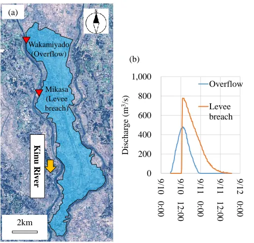
In September 2015, disastrous flooding occurred along the Kinu River. The flooding was caused by intensive rainfall in central Japan [8]. The inundation area as delineated by Matsumoto et al. [8] is shown in Figure 2a. This inundation area was extended by overflow at Wakamiyado and a levee breach at Mikasa (Figure 2a). Niroshinie et al. [14] presented the flooding hydrograph at these two points (Figure 2b). We used this hydrograph as input data for the inundation simulation. The calculated inundation area and its increase with the time are shown in Figure 3. According to field observations by Niroshinie et al. [14], the inundation depth ranged from 0.5–2.0 m near Wakamiyado and reached a depth of 3.0 m near Mikasa. Our results agree with these trends (Figure 3). In addition, the maximum inundation area was similar for the observation and simulation studies (Figure 2a, 3). These results indicate that FLOOD View is able to evaluate the scale and the potential risk of flood sufficiently accurately. However, there was a small difference between the observation and simulation values at the southern inundation front (Figure 2a, 3). Although there is a small river that is used for rice cultivation within the inundation area, the DEM (consisting of 10-m mesh data in this study) could not represent the river cross-section correctly. Niroshinie et al. [14] coupled a 1D model representing the impact of the river with a 2D inundation model for this flood. The present study did not attempt to rectify the effects of the coarse mesh in such a way. Thus, the discrepancy between the observation and simulation values in the present study could be caused by the coarse mesh used.
3.2
Debris flow disaster
In August 2014, Hiroshima experienced heavy local rain exceeding 200 mm in 3 hrs, which caused 75 debris flow disasters and the loss of 73 lives [9]. We selected one of the largest events to validate our system. An aerial photograph after the disaster is shown in Figure 4a. We also show the bed
Figure 1: Outline of FLOOD View. Extract the target domain
Input roughness coefficient, hydrograph, etc. Input lat/lon
deposition height at the residential area in Figure 4b that was observed by the Chugoku Regional Branch of the Japan Society of Civil Engineers [9]. To determine debris inflow conditions (Eq. (8) and (9)), a value for A was obtained using FLOOD View (Figure 4c), and P24 was set to the observed precipitation
before the disaster. Figures 5a and 5b represent the deposited height of sediment and the maximum water depth from the initial bed surface elevation, respectively. According to a field survey report [9], the maximum deposited height was about 3 m, and sediment was not deposited beyond the railway line. The calculated distribution of deposited sediment (Figure 5a) was consistent with these observations.
Figure 2: Kinu River flooding inundation in September 2015: (a) Inundation area [8], and (b) Flood hydrograph [14].
Ki
nu
River
Wakamiyado (Overflow)
Mikasa (Levee breach)
0 200 400 600 800 1,000
9/10 0:00 9/10 12:00 9/11 0:00 9/11 12:00 9/12 0:00
Dis
cha
rge (m
3/s)
Overflow
Levee breach (a)
(b)
2km
Figure 3: Changes in inundation area with time.
9/10 11:00 9/10 14:00 9/10 17:00 9/10 19:00 9/10 23:00 Maximum
Furthermore, another report showed that the maximum water level extended across the railway line [15], which also supports our results. Therefore, we consider that FLOOD View is sufficiently accurate for evaluating the scale and the potential risk of debris flow. However, the distribution of deposited sediment showed a small difference between the observed and the simulated results for the residential area (Figure 4b, 5a). The debris flow actually split before reaching the residential area [9], although this trend was not shown in our results. This discrepancy may arise from the use of the coarse computational mesh that cannot represent detailed geography such as roads and houses. For example, Nakatani et al. [16] simulated this debris flow event by applying a 2D debris-flow model with 2-m mesh data, including information on roads and houses, and replicated the sediment deposition at the housing area exactly.
Figure 4: Debris flow disaster in Hiroshima in August 2014: (a) Aerial photograph after the disaster [13], (b) Observed deposition height at residential area [9], and (c) Catchment area obtained by FLOOD View.
(a) (b)
30m
1m > 0.5m > 0.1m > 0.01m >
100m
(c)
Figure 5: Results of debris flow simulation: (a) Deposition height, and (b) Maximum water depth.
(m) (m)
3.3
Complex flood and debris flow disasters
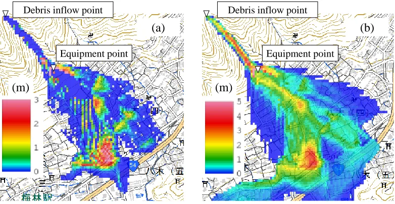
In the present study, FLOOD View predicted an actual flood and debris flow event favorably. Therefore, we proceeded to simulate a flood of hydropower equipment triggered by a debris flow disaster as a case study. In this scenario, we used the same debris flow event as used in the last section, and added a set of hydropower equipment that would be impacted by debris flow (Figure 6a). A time series of fluid force was calculated using debris flow depth and velocity (Figure 6b). According to Figure 6b, debris flow reached the equipment 130 s after the occurrence of debris flow. This impact
Figure 6: Complex flood and debris flow disaster: (a) Water depth after 130 s from the occurrence, and (b) Fluid force at the equipment.
(m)
0.0 5.0 10.0 15.0 20.0
0 500 1,000
Fluid
force (
kN
/m
2)
Time (s) Debris inflow point
Equipment point
(b) (a)
Figure 7: Results of complex disaster simulation: (a) Deposition height, and (b) Maximum water depth.
(m)
(a)
(m)
(b)
Debris inflow point Debris inflow point
caused damage to the equipment and then a flood occurred as the equipment discharged at a rate of 100 m3/s for 1,800 s. FLOOD View allowed us to simulate this additional inflow by inputting this
hydrograph at the equipment point. This inflow was treated as debris flow with no sediment concentration (i.e., cs = 0 in Eq. (2)). Thus, this inflow had the ability to cause erosion and deposition
on the bed surface. Figures 7a and 7b represent the deposited height of sediment and the maximum water depth from the initial bed surface elevation, respectively. Comparing Figure 5a with Figure 7a, we identified sediment movement and increased sediment thickness. Furthermore, the inundation area increased significantly (Figure 5b, 7b). These results indicate the importance of constructing a debris barrier to prevent accidental floods. The results also show that FLOOD View is able to satisfactorily predict complex flood and debris flow disasters.
4
Conclusions
We developed FLOOD View to efficiently simulate flood and debris flow by using a 2D raster-based diffusion wave model. In addition, this system draws on DEM data throughout Japan to create an exact target domain. We applied this system to actual flood and debris flow disasters, and validated it by comparing the results with observed data. Although FLOOD View had difficulty in predicting the impact of micro-topography as a result of the coarse mesh data, overall it satisfactorily represented the scale and potential risk of these disasters. We also conducted a case study to predict a complex flood and debris flow disaster. The results showed a significant increase in the extent of the inundation area in comparison to debris flow alone, which indicates the importance of appropriate countermeasures. These results indicate that FLOOD View is a practical and sufficiently accurate system for simulating flood flow, debris flow, and a combination of the two.
References
[1] S. Toda, R.S. Stein, P.A. Reasenberg, J.H. Dieterich, A. Yoshida, Stress transferred by the 1995 Mw = 6.9 Kobe, Japan, shock: Effect on aftershocks and future earthquake probabilities. Journal of
Geophysical Research, 103(B10), 24,543–24,565, 1998.
[2] R.H. Sibson, An episode of fault-valve behaviour during compressional inversion? – The 2004 MJ 6.8 Mid-Niigata Prefecture, Japan, earthquake sequence. Earth and Planetary Science Letters, 257,
188–199, 2007.
[3] A. Kato, K. Obara, T. Igarashi, H. Tsuruoka, S. Nakagawa, N. Hirata, Propagation of Slow Slip Leading Up to the 2011 Mw 9.0 Tohoku-Oki Earthquake. Science, 335(6069), 705–708, 2012.
[4] Y. Kajitani, K. Yamamoto, Y. Toyoda, M. Nakajima, Survey on past damage records of waterpower plans and investigation on estimation methodology of social impacts caused by the overflow water. Journal of Japan Society of Civil Enginieers, F4, 67(1), 1–13, 2011 (in Japanese).
[5] D. Yu, Diffusion-Based Flood Inundation Modelling. VDM Verlag Dr. Mueller, 2010.
[6] M.S. Horritt, P.D. Bates, Predicting floodplain inundation: raster-based modelling versus the finite-element approach. Hydrological Processes, 15, 825–842, 2001.
[7] D. Rickenmanna, D. Laiglec, B.W. McArdella, J. Hüblb, Comparison of 2D debris-flow simulation models with field events. Computational Geosciences, 10, 241–264, 2006.
[9] Japan Society of Civil Engineers Chugoku regional branch, Investigation report of heavy rain disaster in Hiroshima in Augsut 2014, 2015 (in Japanese).
[10] Z.J. Li, Z.X. Cao, G. Pender, P. Hu, Numerical analysis of adaptation-to-capacity length for fluvial sediment transport. Journal of Mountain Science, 11(6), 1491–1498, 2014.
[11] T. Takahashi, H. Nakagawa, Y. Satofuka, Flood and sediment disasters triggered by 1999 rainfall in Venezuela: A river restoration plan for an alluvial fan. Journal of Natural Disaster Science, 23, 65–82, 2001.
[12] T. Takahashi, Debris flow: Mechanics, Prediction and Countermeasures. Taylor & Francis, Leiden, CRC Press, London, UK, 2007.
[13] Geospatial Information Authority of Japan website, http://www.gsi.go.jp/kibanjoho/kibanjoho40030.html (in Japanese).
[14] M.A.C. Niroshinie, K. Ohtuski, Y. Nihei, Effect of small rivers for the inundations due to levee failure at Kinu River. Procedia Engineering 154, 794–800, 2016.
[15] M. Kaibori, Y. Ishikawa, Y. Satofuka, K. Matsumura, K. Nakatani, Y. Hasegawa, N. Matsumoto, T. Takahara, K. Fukutsuka, K. Yoshino, E. Nagano, M. Fukuda, Y. Nakano, T. Shimada, D. Hori, T. Nishikawa, Sediment-related disasters induced by a heavy rainfall in Hiroshima-city on 20th August, 2014, Journal of the Japan Society of Erosion Control Engineering, 67(4), 49–59, 2014 (in Japanese).

![Figure 4: Debris flow disaster in Hiroshima in August 2014: (a) Aerial photograph after the disaster [13], (b) Observed deposition height at residential area [9], and (c) Catchment area obtained by FLOOD View](https://thumb-us.123doks.com/thumbv2/123dok_us/8878269.1818163/6.612.120.480.347.494/disaster-hiroshima-photograph-observed-deposition-residential-catchment-obtained.webp)