Vol. 5, No. 2, 2013 Article ID IJIM-00213, 5 pages Research Article
Legendre polynomials for numerical solution of linear fuzzy Fredholm
integral equations
P. Salehi∗ † , M. Nejatiyan‡
————————————————————————————————–
Abstract
In this paper, a numerical method is proposed for solving the fuzzy linear Fredholm integral equations of the second kind. For this result, we choose Legendre polynomials as basis functions and collocation method to estimate a solution for an unknown function in these equations. Finally, a numerical example will be stated to illustrate this method.
Keywords: Fuzzy number; Fuzzy Fredholm integral equation; Collocation method; Legendre polyno-mials.
—————————————————————————————————–
1
Introduction
I
nbeen proposed for solving fuzzy linear inte-recent years, many numerical methods have gral equations. For example, in [10], the au-thors used the divided differences and finite dif-ferences methods for solving a parametric of the fuzzy Fredholm integral equations of the second kind. Also, in [9], a numerical method is proposed for the approximate solution of fuzzy linear Fred-holm functional integral equations of the second kind by using iterative interpolation. Moreover, in [2], a numerical procedure is proposed for solv-ing the fuzzy linear Fredholm integral equations of the second kind by using Lagrange interpo-lation based on the extension principle. In [7], the classic Galerkin method for solving integral equations of the second kind was improved to fuzzy Galerkin method, and, the error analysis, namely, error estimate, stability and convergence∗Corresponding author. [email protected] †Department of mathematics, Hamedan Branch, Is-lamic Azad University, Hamedan, Iran.
‡Department of mathematics, Science and Research Branch, Islamic Azad University, Tehran, Iran.
of the extended method were discussed and some results were established. In [5], the homotopy analysis method (HAM) was applied for solving fuzzy linear Fredholm integral equations of the second kind. The results revealed the validity and the great potential of HAM in solving fuzzy inte-gral equations.
In this paper, after converting the following fuzzy integral equation
F(t) =g(t)+(F H) ∫ b
a
k(t, s)F(s)ds ; t∈[a, b]
to the two crisp equations, we use the procedure proposed in [8] and approximate the unknown function.
The important point is that, we haven’t used the technic of fuzzy linear system introduced in [3].
2
Preliminaries
Definition 2.1 [6] A fuzzy number is a function
u:ℜ −→[0,1] having the properties:
(i) u is normal, that is ∃x0∈ ℜ withu(x0) = 1;
(ii) u is fuzzy convex set (that is u(λx+ (1− λ)y) ≥ min{u(x), u(y)} ∀x, y ∈ ℜ λ ∈ [0,1]);
(iii) u is upper semi-continuous onℜ;
(iv) the support{x∈ ℜ:u(x)>0}is a compact set.
The set of all fuzzy real numbers is de-noted by ε1. For 0 < α ≤ 1, let us define [u]α = {x∈ ℜ:u(x)≥α} and [u]0 = {x∈ ℜ:u(x)>0}. Also, we define uα
− = inf [u]α and uα+ = sup [u]α.
For u, v ∈ ε1 and λ ∈ ℜ, we have the sum u + v and the product λu defined by [u+v]α = [u]α+ [v]α, [λu]α =λ[u]α ∀α ∈[0,1], where [u]α + [v]α means the usual addition of two intervals (as subsets ofℜ), andλ[u]α means
the usual product between a scaler and a subset of ℜ. We denote by ∑ the sum of real numbers and also the sum of fuzzy numbers with respect to + (if the terms are fuzzy numbers).
Also, we use the Hausdorff distance between fuzzy numbers given byd∞:ε1×ε1 −→ ℜ+∪{0}. as in [4]
d∞(u, v) = sup
α∈[0,1]
{dH([u]α,[v]α)}
= sup
α∈[0,1]
max{|uα−−v−α|,|uα+−v+α|}
where [u]α = [uα−, uα+],[v]α = [v−α, vα+] ⊆ ℜ and dH is the Hausdorff distance. We define ||.||F=d∞(.,o).˜
Then we have the following theorem and it is known.
Theorem 2.1 See [1]
(i) ||.||F has the properties of a usual norm on
ε1 i.e ||u||F=o iff u= ˜o,
||λu||F= |λ|||u||F, and ||u + v||F≤ ||u||F+||v||F.
(ii) | ||u||F−||v||F |≤ d∞(u, v) and
d∞(u, v)≤ ||u||F+||v||F for any u, v∈ε1.
The following theorem is very important in concept of distance between fuzzy numbers:
Theorem 2.2 See [11]
(i) (ε1, d
∞) is a complete metric space.
(ii) d∞(u+v, v+w) =d∞(u, w) ∀u, v, w∈ε1
(iii) d∞(λu, λv) =|λ|d∞(u, v) ∀u, v∈ε1, ∀λ∈
ℜ
(iv) d∞(u + v, w + e) ≤ d∞(u, w) + d∞(v, e) ∀u, v, w, e∈ε1
In [11] Congxin Wu and Zengtai Gong intro-duced the concept of the Henstock integral for a fuzzy-number-valued function.
Let f : [a, b] −→ ε1. For ∆n : a = x0 <
x1 < ... < xn = b a partition of the interval
[a, b], let us consider the intermadiate points ζi ∈ [xi−1, xi], i = 1, ..., n , and δ : [a, b]−→ ℜ+.
The division P = {([xi−1, xi];ζi);i = 1, ..., n}
denoted shortly by P = (∆n, ζ) is said to be
δ−f ineif:
[xi−1, xi]⊆(ζi−δ(ζi), ζi+δ(ζi)).
The function f is called Henstock integrable to I ∈ ε1 if for every ϵ > 0 there is a function δ : [a, b]−→ ℜ+such that for anyδ−f inedivision P we have:
d∞(Σni=1(xi−xi−1)f(ζi), I)< ϵ.
ThenI is called the Henstock integral off and it is denoted by:
(F H) ∫ b
a
f(t)dt.
If the above δ : [a, b]−→ ℜ+ is constant func-tion, then one recaptures the concept of Riemann integral introduced by Goestchel and Voxman [6]. In this caseI ∈ε1 will be called the Riemann in-tegral off on [a, b] and will be denoted by:
(F R) ∫ b
a
f(t)dt.
Theorem 2.3 See [11]
(i) If f and g are Henstock integrable mapping and if d∞(f(t), g(t)) is Lebesgue integrable, then:
d∞( (F H) ∫ b
a
f(t)dt , (F H) ∫ b
a
Table 1: The values of (sj, P6(F(sj, αr) )) for the membership degrees of αr= 0,1, ...,5.
r0= 0 r1= 0.2 r2= 0.4 r3= 0.6 r4= 0.8 r5= 1
sj
-1 0 0.2819 0.5639 0.8458 1.1277 1.4096
-0.8333 0 0.2968 0.5936 0.8904 1.1872 1.4839
-0.6667 0 0.3143 0.6287 0.9430 1.2574 1.5717
-0.5 0 0.3351 0.6702 1.0052 1.3403 1.6754
-0.3333 0 0.3596 0.7192 1.0787 1.4383 1.7979
-0.1667 0 0.3885 0.7770 1.1656 1.5541 1.9426
0 0 0.4227 0.8454 1.2681 1.6908 2.1135
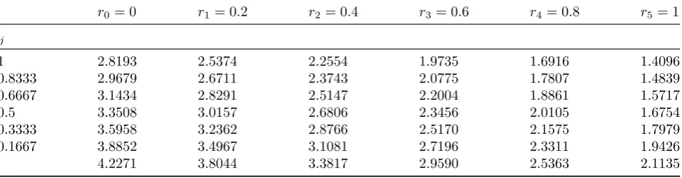
Table 2: the values of (sj, P6(F(sj, αr) )) for the membership degrees ofαr= 0,1, ...,5.
r0= 0 r1= 0.2 r2= 0.4 r3= 0.6 r4= 0.8 r5= 1
sj
-1 2.8193 2.5374 2.2554 1.9735 1.6916 1.4096
-0.8333 2.9679 2.6711 2.3743 2.0775 1.7807 1.4839
-0.6667 3.1434 2.8291 2.5147 2.2004 1.8861 1.5717
-0.5 3.3508 3.0157 2.6806 2.3456 2.0105 1.6754
-0.3333 3.5958 3.2362 2.8766 2.5170 2.1575 1.7979
-0.1667 3.8852 3.4967 3.1081 2.7196 2.3311 1.9426
0 4.2271 3.8044 3.3817 2.9590 2.5363 2.1135
∫ b
a
d∞(f(t), g(t))dt.
(ii) Let f : [a, b]−→ε1 be a Henstock integrable bounded mapping. Then for any fixed u ∈ [a, b], the functionφu : [a, b]−→ ℜdefined by
φu(t) =d∞(f(u), f(t))is Lebesgue integrable on[a, b].
3
Numerical method
Consider the fuzzy linear Fredholm integral equation of the second kind:
F(t) =g(t)+(F H) ∫ b
a
k(t, s)F(s)ds ; t∈[a, b]
(3.1) wherek: [a, b]×[a, b]−→ ℜ and g: [a, b]−→ε1 are known functions, but F : [a, b]−→ε1 is an unknown function. Considering the nonnegative kernel k , the above fuzzy equation replaced by the two following crisp equations
F(t, α) =g(t, α) + ∫ b
a
k(t, s)F(s, α)ds; α∈[0,1]
(3.2)
and
F(t, α) =g(t, α) + ∫ b
a
k(t, s)F(s, α)ds;α∈[0,1].
(3.3) The Legendre polynomials Lm(t) on the interval
[−1,1] are given by the following recursive for-mula.
L0(t) = 1
L1(t) = t
Lm+1(t) =
2m+ 1
m+ 1 tLm(t)
− m
m+ 1 Lm−1(t) m= 1,2,3, ...
We estimate the two unknown functions F(t, α), F(t, α) through the following Legendre polynomials.
F(t, α)≈Pm(F(t, α) ) = m
∑
i=0
aiαLi(t) (3.4)
and
F(t, α)≈Pm( F(t, α) ) = m
∑
i=0
0.7675 -0.9028 0.6851 -0.4164 0.2533 -0.1365 0.0604
0.7253 -0.7185 0.3829 -0.0981 -0.0043 0.0721 -0.0876
0.6755 -0.5310 0.1368 0.0808 -0.0768 0.0164 0.0593
A= 0.6166 -0.3398 -0.0529 0.1479 -0.0476 -0.0839 0.1264
0.5471 -0.1440 -0.1863 0.1310 0.0185 -0.1202 0.0597
0.4649 0.0570 -0.2631 0.0576 0.0750 -0.0670 -0.0517
0.3679 0.2642 -0.2832 -0.0446 0.0940 0.0453 -0.1037
By using (3.4) and (3.5) in the equations (3.2) and (3.3)
m
∑
i=0
aiαLi(t) =g(t, α) +
∫ b
a
k(t, s)
m
∑
i=0
aiαLi(s)ds,
(3.6) α ∈[0,1].
and
m
∑
i=0
aiαLi(t) =g(t, α) +
∫ b
a
k(t, s)
m
∑
i=0
aiαLi(s)ds,
(3.7) α∈[0,1].
So, we define the residual equations the given form
Rm(t) =
m
∑
i=0
aiαLi(t)−g(t, α)−
∫ b
a
k(t, s)
m
∑
i=0
aiαLi(s)ds
(3.8) and
Rm(t) =
m
∑
i=0
aiαLi(t)−g(t, α)−
∫ b
a
k(t, s)
m
∑
i=0
aiαLi(s)ds.
(3.9) To determine the unknown coefficients aiα, aiα,
we choose some points of collocation as
Rm(sj) =Rm(sj) = 0 ; j= 0,1, ..., m.
Such as [8] collocation points are
sj =a+
(b−a)
m j ; j= 0,1, ..., m.
Therefore, we have two linear systems of equa-tions
AmXα=bmα , AmXα=bmα
in which
Am = [ Li(sj)−
∫b
ak(sj, s)Li(s)ds ] m
j=0 ; i = 0,1, ..., m
XαT = [ aiα ]mi=0 , bm = [g(sj, α)] ; j =
0,1, ..., m
Xα T
= [ aiα ]mi=0 , bm = [g(sj, α)] ; j =
0,1, ..., m.
For investigating convergence of procedure and its speed you can refer [8].
Example 3.1 Consider the following fuzzy inte-gral equation
F(t) = (0,1,2)+(F H) ∫ 0
−1
et+sF(s)ds ; t∈[−1,0]
where, (0,1,2) is a triangular fuzzy number with level sets as:
[(0,1,2)]α= [α,2−α].
Therefore, using parametric representation of fuzzy numbers, we have
F(t, α) =α+ ∫ 0
−1
et+sF(s, α)ds ; α∈[0,1]
and
F(t, α) = 2−α+ ∫ 0
−1
et+sF(s, α)ds ; α∈[0,1].
Choosing αr= 15r ; r= 0,1, ...,5 and collocation points as
sj =−1 +
1
6j ; j = 0,1, ...,6
we can use Legendre polynomials
L0(t), L1(t), ..., L6(t) to approximate unknown
4
Conclusion
The aim of this paper, is to propose a simple nu-merical method to solve linear fuzzy Fredholm in-tegral equations with nonegative kernels. In this method, we use Legendre polynomials to approx-imate the unknown functions of crisp linear in-tegral equations obtained from the fuzzy inin-tegral equation. Such a method for crisp equations has been used in [8] and the convergence of its was investigated there.
References
[1] G. A. Anastassiou, S. G. Gal, On a fuzzy trigonometric approximation theorem of Weierstrass-type, J. Fuzzy Math. 9 (2001) 701-708.
[2] M. A. Fariborzi Araghi, N. Parandin, Nu-merical solution of fuzzy Fredholm integral equations by the Lagrange interpolation based on the extension principle, Soft computing. Springer-Verlag 15 (2011) 2449-2456.
[3] M. Friedman, M. Ming, A. Kandel, Fuzzy linear systems, Fuzzy Sets and Systems 96 (1998) 201-209.
[4] S. G. Gal,Approximation theory in fuzzy set-ting, in: G. A. Anastassiou (Ed.), Handbook of Analytic-Computational Methods in applied Mathematics, Chapman & Hall, CRC Press, Boca Raton, London, New York, Washington DC, (2000) (Chapter 13).
[5] Mojtaba Ghanbari, Approximate Analytical Solutions of Fuzzy Linear Fredholm Integral Equations by HAM, International Journal of Industrial Mathematics 4 (2012) 53-67.
[6] R. Goetschel, W. Voxman, Elementary fuzzy calculus, Fuzzy Sets and Systems 18 (1986) 31-43.
[7] Taher Lotfi, Katayoun Mahdiani, Fuzzy Galerkin Method for Solving Fredholm Inte-gral Equations with Error Analysis, Interna-tional Journal of Industrial Mathematics 4 (2011) 237-249.
[8] K. Maleknejad, K. Nouri, M. Yousefi, Discus-sion on convergence of Legendre polynomial for numerical solution of integral equations,
Applied Mathematics and Computation 193 (2007) 335-339.
[9] N. Parandin, M. A. Fariborzi Araghi,The ap-proximate solution of linear fuzzy Fredholm integral equations of the seconde kind by us-ing iterative interpolation, World academy of science. Engineering and technology 49 (2009) 978-984.
[10] N. Parandin, M. A. Fariborzi Araghi, The numerical soluton of linear fuzzy Fredholm in-tegral equations of the second kind by using fi-nite and divided differenes methods, Soft com-puting. Springer-Verlag 15 (2010) 729-741.
[11] C. Wu, Z. Gong, On Henstock integral of fuzzy-number-valueed functions, Fuzzy Sets and Systems 120 (2001) 523-532.
Parham Salehi was born in 21 sep 1983. He has M.Sc degree in applied mathematics from Is-lamic Azad university, science and research branch in Tehran in sep 2010. He is interested in fuzzy mathematics and numerical anal-ysis especially: approximation theory, integral equations, differential equations.