A Recurrent Neural Network for Solving Strictly Convex Quadratic Programming Problems

(1)

Vol. 10, No. 4, 2018 Article ID IJIM-01083, 9 pages Research Article

A Recurrent Neural Network for Solving Strictly Convex Quadratic

Programming Problems

A. Ghomashi ∗†, M. Abbasi‡

————————————————————————————————–

Abstract

In this paper, we present an improved neural network to solve strictly convex quadratic program-ming(QP) problem. The proposed model includes a set of differential equations such that their equi-librium points correspond to optimality condition of convex (QP) problem and has a lower structure complexity respect to the other existing neural network model for solving such problems. In theoret-ical aspect, stability and global convergence of the proposed neural network is proved. The validity and transient behavior of the proposed neural network are demonstrated by using four numerical examples.

Keywords: Dynamical system; Strictly convex quadratic programming; Stability; Global convergence; Recurrent neural networks

—————————————————————————————————–

1 Introduction

O

nmization problems with hight dimension ande promising approach to solving the opti-dense structure in real time is to employ artifi-cial neural networks based on circuit implemen-tation [24]. Neural networks are computing sys-tems composed of a number of highly intercon-nected simple information processing units, and thus can usually solve optimization problems in execution times at the orders of magnitude much faster than most popular optimization algorithms for general-purpose digital [24]. A neural net-work with a good computational performance should satisfy threefold. First, the global conver-gence of the neural networks with an arbitrarily given initial state should be guaranteed. Second,

∗_{Corresponding author.} _{a ghomashi [email protected],} Tel:+98(918)7260024.

†_{Department of Mathematics, Kermanshah Branch,} Is-lamic Azad University, Kermanshah, Iran.

‡_{Department of Mathematics, Kermanshah Branch,} Is-lamic Azad University, Kermanshah, Iran.

the network design preferably contains no vari-able parameter. Third, the equilibrium points of the network should correspond to the exact or approximate solution [17]. Solving optimiza-tion problems using recurrent neural networks has fascinated much attention since seminal work of Tank and Hopfield [11]. Many neural network for constrained optimization problems has been developed during the past two decades,e.g.see [2, 3, 4, 6, 7, 8, 9, 10, 12, 13, 15, 17, 18, 19,

20,21, 22,24,26,28,30] and references therein. Kennedy and Chua [4] presented a neural net-work for solving the strictly convex quadratic pro-gramming. Proposed model by kennedy and chua contain a finite penalty parameter, thus their model converges to an approximate optimal solu-tion. Lately, many researchers successively pro-posed a number of primal-dual neural networks [8,9,28] and projection neural networks for solv-ing linear and quadratic programmsolv-ing problems [2,6,15,18,20,23,24,26]. Moreover, a number of neural networks models proposed for solving a

(2)

special forms of quadratic programming problems such asL1-norm estimation andL2-norm estima-tion problems [14,16,25]. These neural networks were proved to be globally convergent to the ex-act solutions.

We are concerned with the following QP problem:

MinimizecTx+1₂xTQx

subject to ¯

l≤Ax≤¯h l≤x≤h

(1.1)

where c, x ∈ Rn, A ∈ Rm×n,¯l and ¯h ∈ Rm,

Rank(A) = m and Q ∈ Rn×n _{is symmetric and}

positive definite matrix.

Problem (1.1) is a general form of quadratic pro-gramming problem. In the most of existing neu-ral network models for solving (1.1), constraint ¯

l≤Ax≤¯hdivided two part, ¯l≤AxandAx≤¯h, thus dimension of problem increases. First time, Xia et al. studied [22] a neural network for solving (1.1) without dividing ¯l≤Ax≤¯h into two part. Proposed model in [22] motivates us to propose a neural network model with one layer structure for solving (1.1) with lower model complexity respect to proposed model in [22]. The proposed neural network is shown to to be globally convergent to unique exact solution of (1.1)within a finite time. Simulation results show that the proposed neu-ral network is effective for solving strictly convex quadratic programming problems. This paper is divided into six sections. In next section prelim-inary information is introduced to facilitate later discussions. In section III, first we present that problem (1.1) is equivalent with solving a piece-wise equation and then introduce a neural net-work model for solving this piecewise equation. In section IV, we analyze stability condition and global convergence. In section V, illustrative ex-amples are discussed. Section VI gives the con-clusion of this paper.

2 Preliminaries

Definition 2.1 Let X = {x ∈ Rm|li ≤ xi ≤

ui,∀i ∈ N ⊆ L} where L = {1,2, ..., m}, PX :

Rm_→_X _{is a projection operator to set}_X_defined

by

PX(x) =arg min ∥x−y∥ y ∈X

Where∥.∥denotes thel2-norm of Rm [24]. Since

X is a box set, PX(x) can be presented by

PX(x) = [PX(x1), ..., PX(xm)]T, where for i ∈

L−N, PX(xi) =xi and fori∈N

PX(xi) =

  

li, xi< li xi li ≤xi ≤ui ui xi> ui

(2.2)

Lemma 2.1 [5] For all y ∈ Rm and all x ∈ X ⊆Rm

(y−PX(y))T(PX(y)−x)≥0

and for x, y∈Rm

∥PX(x)−PX(y)∥≤ ∥x−y∥

Definition 2.2 The finite-dimensional

varia-tional inequality problem V I(F, K) is to

deter-mine a vector x∗ ∈K ⊆Rn, such that

F(x∗)T(x−x∗)≥0, ∀x∈K

where F is a given continuous function from K

to Rm, K is a given closed convex set [5].

Theorem 2.1 [5] Assume that K is closed and

convex. Then x∗ ∈ K is a solution of the

varia-tional inequality problem V I(F, K) if and only if

for any γ >0

PK(x∗−γF(x∗)) =x∗

Let f : Rn → Rn, now we introduce some basic properties of the following differential equation:

˙

x(t) =f(x(t)), x(t0)∈Rn (2.3)

Theorem 2.2 [29] Assume that f in (2.3) is

a continuous mapping, then for arbitrary t0 ≥ 0

and x0 ∈Rn there exists a local solution x(t) to

(2.3) where t ∈ [t0, τ] for some τ > t0.

Fur-thermore if f is locally Lipschitzian continuous

atx0 then the solution is unique, and if f is

Lip-schitzian continuous inRnthenτ can be extended

to +∞.

Theorem 2.3 [29] Let x∗ is an equilibrium

point of (2.3) and X ⊂ Rn be an open

neigh-borhood of x∗, if V : Rn → R is a continuously

differentiable function over X and V satisfies in

the following conditions:

(3)

• dV(x(t))

dt ≤0, V(x)>0, ∀x∈X− {x∗} • ∥x∥→ ∞ ⇒ ∥V(x)∥→ ∞

then x∗ is a lyapunov stable equilibrium and the

solution always exist globally,if

dV(x(t))

dt <0 ∀x∈X− {x∗}

thenx∗ is a globally asymptotically stable

equilib-rium.

Theorem 2.4 [1] Let S be a nonempty open

convex set in Rn, and letf : S → R be

differen-tiable on S then f is strictly convex if and only

if, for each distinctxl, x2 ∈S, we have

(∇f(x2)− ∇f(x1))T(x2−x1)>0

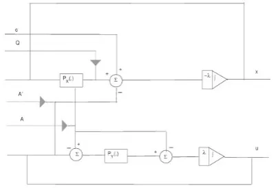
Figure 1: Architecture of the recurrent neural

network (3.7).

3 Neural network model

Throughout this paper, we assume that the fea-sible set of problem(1.1)is nonempty.

The Karush-Kuhn-Tucker conditions of (1.1) has the following form [1]:

Qx+c+ATu= 0, (3.4)

  

(Ax)i= ¯li, ui >0

¯

li ≤(Ax)i ≤¯hi ui = 0

(Ax)i= ¯hi, ui <0

(3.5)

wherex∈X={x∈Rn|l≤x≤h}and u∈Rm.

Lemma 3.1 [21] x¯∈X is an optimal solution

of (1.1) if and only if there existu¯such that(¯x,u¯)

satisfies in (3.4) and (3.5).

¯

x is called a KKT point of (1.1) and ¯u is called the lagrangian multiplier vector corresponding to ¯

x.

Now, let x(.) and u(.) be some time depen-dent variables. In order to use a neural net-work method to solve (1.1), a neural netnet-work sys-tem have to be constructed and make the steady points of neural network system to satisfy the KKT conditions (3.4) and (3.5). By definition 2.1, we can rewrite (3.4) and (3.5) the following form:

{

QPX(x) +c−ATu= 0 PY(APX(x)−u) =APX(x)

(3.6)

where Y = {y ∈ Rm|¯l ≤ y ≤ ¯h},

X = {x ∈ Rn_|_l _≤ _x _≤ _h_}_, _u _∈ _Rm _and x∈Rn.

Using (3.6), we propose a new neural network for solving (1.1) as follows:

dx

dt =−λ(QPX(x) +c−A T_u₎ du

dt =−λ(APX(x)−PY(APX(x)−u))

(3.7)

where λ > 0 is scalar. The architecture of the neural network described in (3.7)is depicted in Figure 1. The system described by Eq.(3.7) can be applied for solving (1.1) with positive definite matrixQand can be easily realized by a recurrent neural network with a one-layer structure.The proposed neural network can be implemented by using a simple hardware only without analog mul-tipliers for the variables or the penalty parame-ter. The operatorPYandPX may be implemented

by using a piecewise activation function. The model contains some amplifiers(PYandPX),

inte-grator, summations, multipliers and interconnec-tions. Among them, the number of amplifiers, integrator and interconnections is important in determining the structural complexity of neural network model.

For comparison purpose, we list the numbers of amplifiers, integrators and interconnections of proposed neural network in (3.7)and proposed neural network in [22] in Table1. we have the fol-lowing observations: 1) the numbers of amplifiers and integrator are same in both models; 2) the proposed model requires fewest interconnections respect to model in [22]. These observations then lead to the conclusion that the proposed model (3.7) is simplest in structure. In what follows, we introduce some basic properties of (3.7).

(4)

Table 1: Comparisons of proposed model and model in [22] for solving (1).

Neural network model Number of amplifiers number of integrator number of interconnections

proposed model m+n m+n n2+ 2mn+ 3n+ 5m

model in [22] m+n m+n (m+n+ 6)(m+n)

of (1.1) where

[ x∗ u∗ ]

denotes the equilibrium point

of (3.7).

Proof. Using lemma 3.1, proof is complete.

Corollary 3.1 Right hand side of (3.7) is Lips-chitz continuous function.

Proof. Let the right hand side of (3.7) be

denoted by L(w), where w = [

x u ]

∈ Rm+n,

by lemma 2.1, for any ˆw = [ ˆ x ˆ u ]

∈ Rm+n, and

¯ w= [ ¯ x ¯ u ]

∈Rm+n, we have:

∥L( ˆw)−L( ¯w)∥= λ    

Q(PX(¯x)−PX(ˆx)) +AT(ˆu−u¯)

PY(APX(ˆx)−uˆ)−PY(APX(¯x) −u¯) +A(PX(¯x)−PX(ˆx))

    ≤ λ    

Q(¯x−xˆ) +AT(ˆu−u¯)

A(PX(ˆx)−PX(¯x))

+ ¯u−uˆ−A(ˆx−x¯)     ≤λ (

Q(¯x−xˆ) +AT(ˆu−u¯) ¯

u−uˆ

)

≤λ (

−Q AT

0 −I

) ( ˆ

x−x¯ ˆ

u−u¯ )

≤λ (

−Q AT

0 −I

) ( xˆ

ˆ u ) − ( ¯ x ¯ u ) Which gives the desired results.

Lemma 3.2 For each initial point

[ x(t0)

u(t0) ]

∈

Rm+n, there exist a unique continuous solution

[ x(t)

u(t) ]

∈Rm+n(t∈[t0, τ))for (3.7) and the equi-librium of neural network in (3.7) correspond to unique optimal solution of (1.1).

Proof. Theorem 2.2 and Corollary 3.1 yield a

unique continuous solution [

x(t)

u(t) ]

over [t0, τ)

ex-ist for (3.7). Since the feasible set of problem(1.1) is nonempty and Q is a positive definite matrix

so there exist a unique optimal solution for (1.1) [1], then using theorem 3.1 and (3.7), proof is complete.

4 Convergence Analysis

In this section, we prove globally asymptotically convergent of (3.7).

The neural network in (3.7) is said to be stable in the sense of Lyapunov and globally convergent, globally asymptotically stable, if the correspond-ing dynamic system is so [24].

Theorem 4.1 The proposed neural network in (3.7) is stable in the sense of Lyapunov and is globally asymptotically convergent to the

unique solution of (1.1) if Q is positive definite.

Moreover, the convergence rate of the neural

network in (3.7) increase as λincreases.

Proof. By Lemma 3.2, we know that for each

initial point [

x(t0)

u(t0) ]

∈Rm+n, there exist a unique

continuous solution [

x(t)

u(t) ]

for (3.7). Let [

x∗ u∗ ]

be equilibria point of (3.7), define a lyapunov function below:

V(x(t), u(t)) = 1₂ ∥x(t)−PX(x∗)∥2

+1₂ ∥u(t)−u∗ ∥2, ∀t≥t0,

Let x = x(t) and u =u(t), then time derivative of V along the trajectory of (3.7) as follows:

d

dtV(x, u) = dV dx dx dt + dV du du dt (4.8) We have dV dx dx

dt =−λ(QPX(x) +c−A

T_u₎T₍_x₋_P X(x∗))

Define g(x) = cTx+ 1₂xTQx−uTAx where u is fix scaler. Since Q is positive definite so g(x) is

strictly convex. since [

x∗ u∗ ]

(5)

of (3.7) so∇g(PX(x∗)) =QPX(x∗) +c−ATu∗ =

0, using theorem 2.4 we have

(∇g(x)− ∇g(PX(x∗))T(x−PX(x∗))>0, x̸=PX(x∗)

So

dV dx

dx dt =

−λ(QPX(x) +c−ATu)T(x−PX(x∗))<0, x̸=PX(x∗)

(4.9)

On the other hand by lemma 2.1we have:

(v−PY(v))T(PY(v)−y)≥0, v∈Rm, y∈Y

Letv=APX(x)−u andy=APX(x∗) then

(APX(x)−u−PY(APX(x)−u))T

(PY(APX(x)−u)−APX(x∗))≥0,

∀x∈Rn_, _∀_u_∈_Rm

(4.10)

By using definition2.2and theorem2.1we have:

(u∗)T(y−APX(x∗))≥0, ∀y∈Y

Lety =PY(APX(x)−u) so

(u∗)T(PY(APX(x)−u)−PX(x∗))≥0, ∀x∈Rn, ∀u∈Rm (4.11)

Sum of (4.10) and (4.11) yields:

(APX(x)−u+u∗−PY(APX(x)−u))T

(PY(APX(x)−u)−APX(x∗))≥0, ∀x∈Rn_, _∀_u_∈_Rm

Then

(u−u∗)T

(PY(APX(x)−I(u))

−APX(x))≤

−∥(PY(APX(x)−I(u))−APX(x))∥2

−(u−u∗)T₍_AP

X(x)−APX(x∗))

(4.12)

By using (3.6) we have

PX(x) =Q−1ATu−Q−1c PX(x∗) =Q−1ATu∗−Q−1c

(4.13)

Substitution (4.13) into (4.12) yields

(u−u∗)T

(PY(APX(x)−I(u))−APX(x))≤

−∥(PY(APX(x)−I(u))−APX(x))∥2

−(u−u∗)TAQ−1AT(u−u∗)≤0

(4.14)

Then

dV du

du dt = λ(u−u∗)T

(PY(APX(x)−I(u))−APX(x))≤0

(4.15)

By using(4.8),(4.9) and (4.15) we have

d

dtV(x, u) = dV dx

dx dt +

dV du

du dt <0, ∀(x, u)̸= (PX(x∗), u∗)

So we have

{(x(t), u(t))|t0≤t < τ} ⊂P0

={(x, u)∈Rm+n_|_V₍_{x, u}₎_≤_V₍_x₍_t

0), u(t0))}

On the other hand we have:

V(x, u)≥ 1₂ ∥x−PX(x∗)∥2, V(x, u)≥ 1₂ ∥u−u∗ ∥2

Since P0 is bounded and {(x(t), u(t))|t0 ≤ t < τ} ⊂P0, (x(t), u(t)) is bounded and thusτ =∞.

Moreover

dV(x,u)

dt = 0⇔

{

QPX(x) +c−ATu= 0

PY(APX(x)−u)−APX(x) = 0 ⇔

{ _dx

dt = 0 du dt = 0

So by applying the theorem2.3, we get result that the proposed neural network is globally asymp-totically convergent to the unique solution of (1.1).

Since dV_dt < 0 then we can result that as λ in-creases, the convergence rate of the neural net-work in (3.7) increases. This proof is completed.

2

5 Illustrative examples

In this section, we demonstrate the effectiveness and performance of the proposed neural network model with four illustrative examples. The ordi-nary differential equation solver engaged in ode23 in matlab 2011.

Example 5.1 Consider the following quadratic

programming problem [22]:

Minimize x2₁+x2₂+x1x2−30x1−30x2

subject to ₁₂5x1−x2 ≤ 35₁₂ 5

2x1+x2≤ 35

2

−5≤x1≤5

−5≤x2≤5

(6)

neural network in (3.7) is globally asymptotically stable to x∗. Figure 2 shows the performance of the neural network in (3.7) with a random initial point and four λ.

Example 5.2 Consider the following quadratic

programming problem [22]:

Minimize x2₁+x2₂+ 5x2₃+x1x2

+x1x3−4x1−3x2−2x3

subject to x1+x2+ 2x3 ≤3

3x1−9x2+ 9x3 = 1 0≤x1, x2, x3≤ 4₃

This problem has a unique optimal solutionx∗ = (4₃,7₉,4₉). We use the proposed neural network in (3.7) to solve Example5.2. Figure3and Figure4 display the convergence behavior proposed model in example5.2.

0 0.5 1 1.5 0 1 2 3 4 5 6 Time λ=5 2(a)

trajectories of x(t) and u(t)

0 0.5 1 1.5 0 1 2 3 4 5 6 Time λ=10 2(b)

0 0.5 1 1.5 −1 0 1 2 3 4 5 6

Time

λ=15 2(c)

0 0.5 1 1.5 −1 0 1 2 3 4 5 6

Time

λ=20 2(d) x1, x2 x1, x2

x

1, x2 x1, x2

u2 u1 u1 u 1 u1

u2 u2

u

2

Figure 2: Transient behavior of the neural

net-work in (3.7) in terms of trajectories in Example

5.1.

Example 5.3 Consider the following quadratic programming problem:

Minimize 3x2₁+ 3x2₂+ 4x2₃+ 5x2₄+ 3x1x2

+ 5x1x3+x2x4−11x1−5x4

subject to 3x1−3x2−2x3+ 4x4 = 0

4x1+x2−x3−24x4 = 0

−x1+x2≤ −1

−2≤3x1+x3≤4

This problem has an optimal solution x∗ = (0.5,−0.5,1.5,0)T. We use the proposed neural network in (3.7) to solve Example 5.3. Figure 5.a illustrates the convergence behavior of the l2

0 0.5 1 1.5 −0.5 0 0.5 1 1.5 Time λ=5 3(a)

Trajectories of x(t) and u(t)

0 0.5 1 1.5 −0.5 0 0.5 1 1.5 Time λ=10 3(b)

0 0.5 1 1.5 −0.5 0 0.5 1 1.5 Time λ=15 3(c)

0 0.5 1 1.5 −0.5 0 0.5 1 1.5 Time λ=20 3(d)

x

1 x1

x1 x1

x2

x2 x2

x2

x3 x3

x

3 x3

u1

u1 u1

u 1 u 2 u 2 u 2 u2

net-work in (3.7) in terms fourλand one random

ini-tial point to solve Example5.2.

0 0.2 0.4 0.6 0.8 1 1.2 1.4 0 0.5 1 1.5 0 0.1 0.2 0.3 0.4 0.5 0.6 0.7 0.8 0.9 1 x 1 x 2 x3 x*

net-work in (3.7) in terms of two initial points to solve

Example5.2.

norm error ∥x(t)−x∗∥ based on the neural net-work in (3.7). Figure5.b displays the trajectories of the state trajectories x(t) started from 10 ran-dom initial points.

Example 5.4 Consider the quadratic

program-ming problem (1.1) [22] where

Q=       

2 1 0 . . . 0 1 2 1 . . . 0

..

. ... ... . .. ... 0 . . . 1 2 1 0 . . . 0 1 2

      

(7)

Table 2: Results of (3.7) and proposed model in [22] for Example5.4.

Model iteration 1 iteration 2 iteration 3 iteration 4

CPU Error CPU Error CPU Error CPU Error

model(7) 0.2188 1×10−5 0.2344 8×10−6 0.2188 7×10−6 0.2344 8×10−6

model in [22] 1 3×10−5 0.9844 1×10−5 0.8906 3×10−5 0.8750 2×10−5

0 0.2 0.4 0.6 0.8 1

0 0.5 1 1.5 2 2.5 3 3.5 4

Time (a)

|| x(t)−x

*||

0 0.2 0.4 0.6 0.8 1

0 0.5 1 1.5 2 2.5 3 3.5 4 4.5

Time (b)

|| x(t)−x

*|| λ=50

λ=65

λ=80

λ=100

Figure 5: Convergence behavior of the proposed

model in terms of the norm error ∥x(t)−x∗∥ in

Example 5.3. (a) with one random initial point

and fourλ. (b) with 10 random initial points and

λ= 200.

and

A=



 01 −11 −01 11 −01 11 10 11 11 −01

−1 1 −1 1 0 1 1 0 1 0

 

Optimal solution of the above problem is x∗ = (0.5,−1.5,0,1,−1.5,2,−1,0.5,0,0). We use the neural network in (3.7) to solve this problem. Figure6shows the transient behavior of the pro-posed model in Example 5.4.

For a comparison, we compute this example us-ing the proposed neural network in (3.7) and pro-posed model in [22] in four iteration. The compu-tational results are listed in Table 2. From Table 2, we see that the proposed neural network not only gives a better solution, but also has faster convergence rate than proposed model in [22].

6 Conclusion

In this paper, a recurrent neural network intro-duced for solving strictly convex quadratic pro-gramming problem so it can solve a broad class of the constrained optimization problems. The

0 0.5 1 1.5 2 2.5 3

0 0.5 1 1.5 2 2.5

Time (a)

|| x(t)−x

*||

0 0.5 1 1.5 2 2.5 3

−1.5 −1 −0.5 0 0.5 1 1.5 2 2.5

Time (b)

Trajectories of x(t)

λ=100

λ=200

λ=300

λ=400 _x

3

x₁

x₄

x

2

Figure 6: (a) Convergence behavior of the

pro-posed model in terms of the norm error∥x(t)−x∗∥

in Example5.4with one random initial points and

four λ. (b) Transient behavior of the proposed

model in Example5.4in terms of one random

ini-tial point andλ= 100

proposed model has a lower structure complexity respect to existing models to solve such problem. It is shown here that the proposed neural net-work is stable in the sense of Lyapunov and glob-ally asymptoticglob-ally convergent to the optimal so-lution. Numerical examples are provided to show the performance of the proposed neural network.

References

[1] S. Boyd, L. Vandenberghe, Convex optimiza-tion,Cambridge university press (2004).

[2] X. Hu, Applications of the general projection neural network in solving extended linear-quadratic programming problems with linear constraints, Neurocomputing 72(2004) 1131-1137.

(8)

Neu-ral Networks, IEEE Transactions on 20 (2009) 654-664.

[4] M. P. Kennedy, L. O. Chua, Neural networks for nonlinear programming. Circuits and Systems, IEEE Transactions on 35 (1988) 554-562.

[5] D. Kinderlehrer, G. Stampacchia, An intro-duction to variational inequalities and their applications (Vol. 31),Siam (2000).

[6] Q. Liu, J. Wang, A one-layer projection neural network for nonsmooth optimization subject to linear equalities and bound con-straints. Neural Networks and Learning Sys-tems, IEEE Transactions on 24 (2013) 812-824.

[7] C. Y. Maa, M. A. Shanblatt, Linear and quadratic programming neural network anal-ysis, Neural Networks, IEEE Transactions on 3 (1992) 580-594.

[8] A. Nazemi, A neural network model for solv-ing convex quadratic programmsolv-ing problems with some applications, Engineering

Appli-cations of Artificial Intelligenc 32 (2014)

54-62.

[9] A. Nazemi, M. Nazemi, A Gradient-Based Neural Network Method for Solving Strictly Convex Quadratic Programming Problems,

Cognitive Computation 5 (2014)1-12.

[10] A. Rodriguez-Vazquez, R. Dominguez-Castro, A. Rueda, A., J. L. Huertas, E. Sanchez-Sinencio, Nonlinear switched ca-pacitor neural networks for optimization problems. Circuits and Systems, IEEE

Transactions on 37 (1990) 384-398.

[11] D. Tank, J. J. Hopfield,

Sim-ple’neural’optimization networks: An A/D converter, signal decision circuit, and a linear programming circuit. Circuits and Systems, IEEE Transactions on 33 (1986) 533-541.

[12] X. Y. Wu, Y. S. Xia, J. Li, W. K. Chen, A high-performance neural network for solv-ing linear and quadratic programmsolv-ing prob-lems. Neural Networks, IEEE Transactions on 7(1986) 643-651.

[13] Y. Xia, A new neural network for solv-ing linear and quadratic programmsolv-ing prob-lems, Neural Networks, IEEE Transactions on 7(1996) 1544-1548.

[14] Y. Xia, A Compact Cooperative Recur-rent Neural Network for Computing Gen-eral Constrained Norm Estimators, Signal Processing,IEEE Transactions on 57 (2009) 3693-3697.

[15] Y. S. Xia, J. Wang, On the stability of glob-ally projected dynamical systems,Journal of

Optimization Theory and Applications 106

(2000) 129-150.

[16] Y. Xia, H. Leung, A Fast Learning Algo-rithm for Blind Data Fusion Using a Novel-Norm Estimation, Sensors Journal, IEEE

14 (2014) 666-672.

[17] Y. Xia, J. Wang, A general methodology for designing globally convergent optimization neural networks, Neural Networks, IEEE

Transactions on 9 (1998) 1331-1343.

[18] Y. Xia, J. Wang, A recurrent neural network for solving linear projection equations,

Neu-ral Networks 13 (2000) 337-350.

[19] Y. Xia, J. Wang, Global exponential stabil-ity of recurrent neural networks for solving optimization and related problems, Neural

Networks, IEEE Transactions on 11 (2000)

1017-1022.

[20] Y. Xia, J. Wang, A general projection neu-ral network for solving monotone variational inequalities and related optimization prob-lems, Neural Networks, IEEE Transactions on 15 (2004) 318-328.

[21] Y. Xia, J. Wang, A recurrent neural network for solving nonlinear convex programs sub-ject to linear constraints, Neural Networks,

IEEE Transactions on 16 (2005) 379-386.

[22] Y. Xia, G. Feng, J. Wang, A recurrent neu-ral network with exponential convergence for solving convex quadratic program and re-lated linear piecewise equations,Neural

Net-works 17 (2004) 1003-1015.

(9)

optimization problems with inequality con-straints, Neural Networks, IEEE

Transac-tions on 19 (2008) 1340-1353.

[24] Y. Xia, H. Leung, J. Wang, A projection neural network and its application to con-strained optimization problems.Circuits and Systems I: Fundamental Theory and Appli-cations, IEEE Transactions on 49 (2002) 447-458.

[25] Y. Xia, C. Sun, W. X. Zheng, Discrete-time neural network for fast solving large lin-ear estimation problems and its application to image restoration, Neural Networks and

Learning Systems, IEEE Transactions on23

(2012) 812-820.

[26] X. Xue, W. Bian ,A project neural network for solving degenerate convex quadratic pro-gram,Neurocomputing 70 (2007) 59-66.

[27] Y. Yan, A New Nonlinear Neural Network for Solving QP Problems, In Advances in Neural Networks ISNN 2014 (pp. 347-357),

Springer International Publishing (2014).

[28] Y. Yang, J. Cao, A feedback neural network for solving convex constraint optimization problems, Appl Math Comput. 201 (2008) 50-74.

[29] J. Zabczyk, Mathematical control theory: an introduction,Springer (2009).

[30] J. Zhang, L. Zhang, An augmented la-grangian method for a class of inverse quadratic programming problems, Appl

Math Optim. 61 (2010) 57-83.

Abbas Ghomashi received the MS degrees in Applied Math-ematics from Tarbiat Moallem University of Sabzevar, Sabzevar, Iran in 2004 and PhD degree from Science and Research Branch, Is-lamic Azad University, Tehran, Iran in 2014. Now, he is an assistant profes-sor in Department of Mathematics, Kermanshah Branch, Islamic Azad University, Iran. His re-search interests include Neural Networks, Linear

and nonlinear programming, Data Envelopment Analysis and Interior Point Methods.