99
Does Financial Development Lead to Poverty Reduction in China? Time Series Evidence
Sin-Yu Ho1, Bernard Njindan Iyke2* 1University of South Africa, South Africa
2Deakin University, Melbourne Burwood Campus, Australia [email protected], [email protected], [email protected]
Abstract: The impact of financial development on poverty reduction has received attention in the literature recently. While the connection between financial development and poverty may appear straight forward in theory, in empirics it may be much complicated. This study attempted at empirically assessing the causal links between financial development and poverty reduction in China for the period 1985–2014. The study used the Toda-Yamamoto causality test to avoid pretesting bias that has featured majority of the existing studies. The study utilized two standard proxies for financial development, namely: the domestic private credit by banks as percentage of GDP, and money supply (M2) as percentage of GDP; and a standard proxy for poverty reduction namely: the household final consumption expenditure per capita growth (annual percentage). The study found a bidirectional causal flow between financial development and poverty reduction, implying that the causal flow between these important variables is independent of the proxy for financial development. This means that financial sector reforms and poverty reduction programs are more of “win-win” strategies in the case of China. Therefore policymakers in China should continue to implement robust financial sector reforms and poverty reduction strategies.
Keywords: Financial Development; Poverty Reduction; Toda-Yamamoto Test; China
1. Introduction
Poverty has remained the world greatest challenge. While poverty is found everywhere, it is more prevalent in developing countries. Poverty, as can be found in some of the influential definitions, is the lack of economic resources that is associated with negative social implications (see Mood and Jonsson, 2016). Being poor leaves a person vulnerable to diseases, dangerous social groups, and unfulfilled personal aspirations. Poor people are often socially excluded thereby living stigmatized lives (see Sen, 1983). The economic hardships that come with poverty imply that the poor are not able to have standard lives, participate in leisure activities, or have nutritionally approved consumption patterns (see Galbraith, 1958; Mack and Lansley, 1985; Callan et al., 1993). It is therefore not a surprise that policymakers and powerful international organizations including the World Bank and the United Nations have preoccupied themselves with fighting poverty. The World Bank, in particular, has reiterated that its major priority is to fight poverty (see Birdsall and Londono, 1997). One way policymakers find as a means to fight poverty is through financial inclusion. Economists have long held the view that improvement in financial institutions and intermediaries, as well as their products and services will enhance the inclusion of the poor in financial activities, thereby enhancing their abilities to save and invest properly (see Stiglitz, 1998; Jalilian and Kirkpatrick, 2002). Even if a well-functioning financial system does not directly enhance poverty reduction, economists have argued that it does by promoting economic growth, which in turn opens up avenues for the poor to earn income. This is in line with the trickle-down theory, which argues that financial development can lead to economic growth thereby lifting the masses from poverty due to the wide avenues created by growth. The trickle-down theory has received overwhelming support in the literature (see, for example, World Bank, 1995; Ravallion and Datt, 2002; Dollar and Kraay, 2002).
100
the extensive financial and economic reforms which led to the rapid growth and expansion of the financial sector have pushed down the phenomenon of rural poverty from 30.7% to 1.6% during the period of 1978 to 20071 [United Nations Development Programme (UNDP), 2008]. These statistics show clearly that financial development has been crucial for poverty reduction in China. Formal assessment of the importance of financial development in the reduction of poverty in China has been surprisingly scant in the literature. The few studies that have tried to investigate the links between poverty reduction and financial development in China include Ho and Odhiambo (2011), Ding et al. (2011), Wen et al. (2005), and Park et al. (2004). This is clearly a gap in the literature which is worth addressing. Also, most of the previous studies on China and the rest of the world have employed causality techniques that are vulnerable to pretesting bias. Pretesting bias results when a causality technique requires that we test for stationarity and cointegration. The popular Engle-Granger, Johansen, and ARDL bounds testing approaches entail testing for stationarity and cointegration. Hence, due to the fact that most of the diagnostic tests for non-stationarity and cointegration have low power against the alternative hypotheses, wrong decisions on stationarity and cointegration could lead to biased causality results. Against this backdrop, we re-assess the causal links between poverty reduction and financial development in China using the Toda-Yamamoto causality test. This technique is not prone to pretesting bias, thereby allowing us to report efficient causal estimates (see Takumah and Iyke, 2017; He and Maekawa, 1999).
The study utilized two standard proxies for financial development, namely: the ratio of domestic private sector credit by banks to GDP, and the ratio of money supply (M2) to GDP; and a standard proxy for poverty reduction namely: the household final consumption expenditure per capita growth (annual percentage). The study found a bidirectional causal flow between poverty reduction and financial development, implying that the causal flow between these two is independent of the indicator of financial development. Hence, financial development has played an important role in the reduction of poverty in China; and at some point, the tremendous poverty reduction has led to further growth and expansion of China’s financial sector. This means that financial sector reforms and poverty reduction programs are more of “win-win” strategies in the case of China. Therefore, policymakers in China should continue to implement robust financial sector reforms and poverty reduction strategies. The remaining sections of this study are organized as follows. Section 2 presents an overview of financial development and poverty reduction in China. Section 3 reviews the related literature. Section 4 outlines the methodology and the data. Section 5 reports and discusses the results, while Section 6 concludes the study.
Overview of Financial Development and Poverty Reduction in China
Financial Development in China: In the late 1970s, China started liberalizing her economy by pursuing various structural, institutional, financial and economic reforms. In terms of financial reforms, China has achieved remarkable improvement in the past decades. Before the financial reforms, China was under the mono-bank system, with the People’s Bank of China (PBOC) performing the role of central bank and commercial bank. After all these reforms, the mono-bank system was reformed and diversified into a fully-fledged financial system (see Allen et al., 2005; Hao, 2006; Zhang et al., 2012; Lin et al., 2015). Currently, the financial sector consists of the central bank (namely the PBOC), commercial banks, policy banks, insurance companies, non-bank financial institutions, stock market, and bond market, among others. The banking sector is largely dominated by the five largest commercial banks. These banks are the Agricultural Bank of China, the Bank of China, the Bank of Communications, the Industrial and Commercial Bank of China, and the China Construction Bank (see Lin et al., 2015; Turner et al., 2012). In the 1980s, China pursued a number of financial reforms, including the expansion of the financial sector and monetization of the economy, which were mainly to revitalize the banking institutions (see Lin et al., 2015). As a result of these extensive financial reforms, the financial system experienced a rapid growth of financial intermediaries beyond the scope of the state-owned commercial banks. During this period, regional banks were setup along the coastal areas in the Special Economic Zones. Also, a network of urban credit cooperatives and rural credit cooperatives were established in the rural areas. In addition, the trust and investment corporations, which were categorized as non-bank financial institutions, were formed. These trust and investment corporations performed selected
101
banking and non-banking services, with some restrictions on loan making and sources of deposits (see Allen et al., 2005).
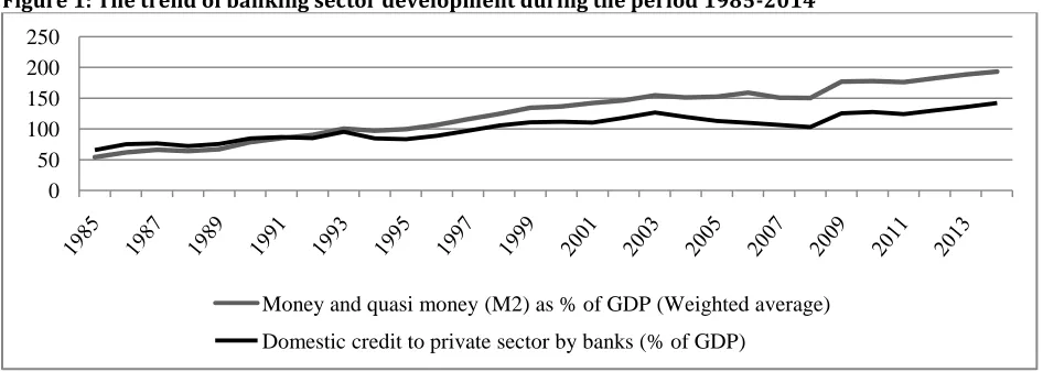
In addition to these early reforms, China undertook a series of banking reforms from 1994 onwards (see Hasan and Zhou, 2006, Zhang et al., 2012; Lin et al., 2015). First of all, three policy banks, namely, the Export-Import Bank of China, the Agricultural Development Bank, and the State Development Bank, were set up in 1994 to relieve the policy lending activities of the state-owned commercial banks. Second, the number of commercial banks was increased by transforming the urban credit cooperatives into city commercial banks, and granting licenses to other non-state commercial banks as well as to some foreign banks. Third, the State control on credit allocation was largely reduced after the abolishment of the credit quota system in 1998. Lastly, the period also witnessed the gradual liberalization of the interest rates. The banking sector has been crucial to China’s remarkable economic growth in the past decades. The early 1980s witnessed a phenomenal financial deepening in China, with the growth of the real monetary balance being faster than the real sector of the economy. The real monetary balance, measured by M2 to GDP, rose from 54% in 1985 to 193% in 2014 (WDI, 2016). This remarkable deepening in the financial sector could be primarily attributed to: (i) the monetization of China’s economy, and (ii) the accumulation of savings of the household. For instance, 77.9% of quasi-money in 2001 was contributed by household deposits. It also accounted for 47.2% of M2 (Hao, 2006). This impressive financial deepening makes China one of the most developed economies. In addition, the growth of the banking sector, as measured by domestic private sector credit by banks to GDP, also showed similar upward trend during the study period. It increased from 66% in 1985 to 142% in 2014 (WDI, 2016). Figure 1 shows the trend of banking sector development during the period 1985-2014.
Figure 1: The trend of banking sector development during the period 1985-2014
Source: World Development Indicators, 2016
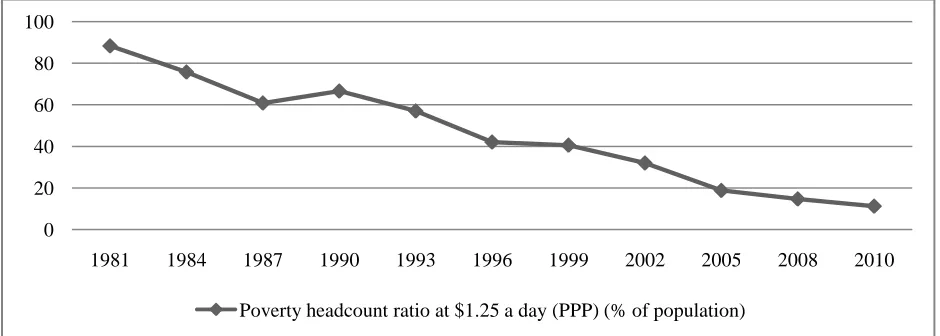
Poverty in China: The pace of poverty reduction in China over the last three decades has been remarkable when measured by various indicators. The rural poverty headcount ratio reduced rapidly from 18.5% to 2.8%, during the period of 1981 to 2004.2 When measured in absolute terms, the number of the rural poverty headcounts declined from 152 million to 26 million during the same period (World Bank, 2009). The figure is even more striking if we use the new international poverty standard of US$1.25 per person per day [2011 purchasing power parity (PPP) for China]. The poverty headcount ratio declined tremendously from 88% to 11%, during the period of 1981 to 2010 (see WDI, 2016). In addition, improvement in other social indicators has been remarkable since the implementation of various economic and social reforms in China. For instance, the average life expectancy at birth improved from 67.3% in 1981 to 75.4% in 2013 (WDI, 2016). Infant mortality rate reduced from 48% in 1980 to 9.2% in 2015 (WDI, 2016). The adult literacy rate improved significantly from 65.5% in 1982 to 95% in 20103 (WDI, 2016). Indeed, poverty in the country is mainly a phenomenon in the rural areas owing to the large disparity in per person income between populations in the urban and rural areas. China has faced a very high incidence of rural poverty in the past. In the early 1980s,
2 These changes are based on China’s official poverty standard of 300 Chinese Yuan per person per year at 1990 prices.
3 The data is available up to year 2010 according to WDI (2016).
0 50 100 150 200 250
Money and quasi money (M2) as % of GDP (Weighted average)
102
the absolute poverty in the rural population was 28%, while it was only 0.3% in the urban population (Wang et al., 2004).However, the extensive economic and social reforms have caused the rural poverty incidence to drop from 30.7% to 1.6% during the period of 1978 to 2007 [United Nations Development Programme (UNDP), 2008]. The China Human Development Report (2008) classifies the country’s poverty reduction policies into four phases.
(i) Phase One: Rural Reform, 1978-1985
This period marked an era of institutional reforms in agricultural activities, procurement prices, and distribution systems. The major institutional reform in the rural areas was the transformation of the collective farming system to the household responsibility system. It significantly incentivized agricultural activities. As a result, the agricultural outputs increased tremendously in China (Lin, 1992). The increase in agricultural output led to the annual growth of per capita net income in rural areas at 16.5% during 1978 to 1985. In addition, the rural poverty headcounts declined rapidly from 250 million to125 million during this period, which witnessed the era of the most significant poverty reduction in the country (UNDP, 2008).
(ii) Phase Two: National Targeted Poverty Reduction Programmes, 1986-1993
During this phase, the government set up task teams and distributed funding for programmes to fight against poverty in the rural areas. As a result of these programmes, the population of the rural poverty head counts declined from 125 million in 1985 to 80 million in 1994 (Wang et al., 2004; UNDP, 2008).
(iii) Phase Three: The Eight-Seven Plan, 1994-2000
The Eight-Seven Plan was introduced by the government in the third phase of poverty reduction programme. The Eight-Seven Plan meant to lift most of the remaining 80 million poor above the official poverty line during the seven-year period of 1994 to 2000. It showed that the poverty reduction programme was expanded to the national level with greater poverty reduction efforts and determination. Due to these efforts, the rural poverty declined from 80 to 32 million during this period (Wang et al., 2004; UNDP, 2008).
(iv) Phase Four: New Century Rural Poverty Alleviation Plan, 2001-2010
During this phase, authorities emphasized the need to re-balance the development gains made across various regions, especially between rural and urban areas. To achieve this aim, China’s Rural Poverty Reduction and Development Compendium (2001–2010) were established in 2001. Its objective was to pursue a balanced poverty reduction strategy in the country, with the focus on developing the central and western regions, and developing the new countryside. As a result, the population of the rural poor fell from 30 to 15 million during the period of 2001 to 2007 (see UNDP, 2008). Figure 2 shows the poverty headcount ratio in China from 1981 to 2010.4
Figure 2: Poverty headcount ratio in China, 1981-2010
Source: World Development Indicators, 2016
4 Data on this indicator is only available from 1981 to 2010 (see WDI, 2016).
0 20 40 60 80 100
1981 1984 1987 1990 1993 1996 1999 2002 2005 2008 2010
103
2. Literature ReviewDoes financial development improve poverty reduction? The literature argues that it does in various ways. First, financial development improves economic and financial avenues for the poor to participate in formal financial activities. This is because financial development addresses the causes of financial market failure including information asymmetry and the high fixed cost of small-scale lending (see, among others, Jalilian and Kirkpatrick, 2002; Stiglitz, 1998). Second, financial development ensures that poor people have access to finance including credit services, which empower their productive assets, and enhance their productivity. Hence, through financial development, poor people are able to have a sustainable livelihood (see Jalilian and Kirkpatrick, 2002; World Bank, 2001). Third, financial development can lead to poverty reduction by promoting economic growth, which is consistent with the trickle-down theory. The trickle-down theory contends that financial development can spur growth thereby lifting the masses from poverty due to the wide avenues created by economic growth. This theory has received overwhelming support in the literature (Dollar and Kraay, 2002; Ravallion and Datt, 2002; World Bank, 1995). Given the theoretical implications of financial development in enhancing poverty reduction, a significant number of studies have been devoted to examining the linkages between the two variables. The available studies can be group into country-specific and panel studies.
Country-specific Studies: The country-specific studies attempting to investigate the linkages between financial development and poverty reduction include but not limited to Abosedra et al. (2016), Sehrawat and Giri(2016a), Uddin et al. (2014), Inoue and Hamori (2012), Ding et al. (2011), Ho and Odhiambo(2011), Geda et al. (2006), Quartey (2005), Wen et al. (2005), Husain (2004), Park et al.(2004), and Burgess and Pande (2003), among others. For example, Sehrawat and Giri (2016a), while examining the link between financial sector development and poverty reduction in India during 1970 to 2012, find financial sector development and economic growth to reduce poverty both in the short and long run. They find a positive and unidirectional causality running from financial development to poverty reduction. Similarly, Abosedra et al. (2016) explore the relationships between financial development and poverty reduction in Egypt by making use of a data set that covers the period 1975Q1 to 2011Q4. They find financial development to reduce poverty. Uddin et al. (2014), while investigating the causal links between financial development, economic growth and poverty reduction in Bangladesh during 1975 to 2011, find a long-run relationship between them. They also find financial development to reduce poverty in nonlinear fashion. Similarly, Inoue and Hamori (2012), while analyzing the importance of financial development in reducing poverty in India, find financial deepening to significantly reduce poverty. Ding et al. (2011) examine the effect of rural financial development on poverty reduction in China using panel data of China's provinces of 2000 to 2008. Their results indicate that rural financial development has both direct and indirect effect on poverty reduction in China. In addition, their results show that the indirect effect was significantly higher than the direct effect. Ho and Odhiambo (2011) find that, in the long run, poverty reduction spurs financial development in China. Also, they find feedback causality between financial development and poverty reduction in the short run in China.
Fairly recent studies have also documented a connection between finance and poverty. For example, Geda et al. (2006), while investigating the relationship between financial development and poverty reduction in Ethiopia from 1994 to 2000, show that access to finance is vital in smoothing consumption and reducing poverty. Quartey (2005) finds financial development to induce poverty reduction in Ghana. Wen et al. (2005) aim at identifying the linkage between the financial development and growth of farmers’ income in China from 1952 to 2003. Their results show that financial development adversely affects the growth of farmers’ income in China. Husain (2004) finds that the reforms implemented in the financial sector during the late 1990s led to pro-poor growth in Pakistan by enabling the poor to access credit from formal institutions. Park et al. (2004) arrive at inconclusive results, while evaluating the effect of micro-finance on poverty reduction in China. Finally, Burgess and Pande (2003), while examining the impact of rural bank branch expansion programme on poverty and output in India during 1977 to 1990, find the programme to have significantly reduced rural poverty, and raised non-agricultural output.
104
Claessens and Feijen (2006), Jalilian and Kirkpatrick (2005; 2002), Honohan (2004), among others. In a very recent study, Sehrawat and Giri (2016b) investigate the importance of financial development in poverty reduction in the case of eleven South Asian developing countries using panel data set over the period of 1990 to 2012. Their empirical results confirm that financial development and poverty reduction are associated in the long run. They find a strong and positive relationship between financial development, trade openness, inflation and poverty reduction. In addition, they find a unidirectional causality running from financial development to poverty reduction. Jeanneney and Kpodar (2008) explore the role of financial development in promoting poverty reduction, and find that the poor benefits from the banking system’s ability to provide savings opportunities and to facilitate transactions – though the poor fails, to some extent, in reaping the benefits made available through the large pool of credit. Their findings suggest that financial development may be linked with financial instability, which may excessively affect the poor negatively. However, they find the benefits associated with financial development to outweigh the costs.
In fairly recent studies, there has been evidence of links between financial development and poverty reduction. Beck et al. (2007), using data on 52 countries from 1960 to 1999, find that on the average income of the lowest quintile increases faster than the average per capita GDP, while income inequality decline more rapidly. Claessens and Feijen (2006) find financial development and improved access to finance to promote economic growth, reduce poverty and undernourishment, and better health, education and gender equality. Jalilian and Kirkpatrick (2005) investigate the impact of financial development on poverty reduction in a group of 42 countries. By employing a pooled panel data approach, they find financial development to contribute to poverty reduction. In an earlier study, Jalilian and Kirkpatrick (2002) investigate the contribution of financial development to poverty reduction in a group of 26 countries. By using a pooled panel data approach, they find a percentage increase in financial development to raise the income growth of the poor in developing countries by nearly 0.4%. Finally, Honohan (2004) investigates the linkage between financial depth and poverty for more than 70 developing countries. He finds that financial depth and poverty are negatively related.
3. Methodology and Data
Data Sources: The data is annual and covers the period 1985 to 2014. The period covered is solely based on data availability. The data is sourced from the World Development Indicators (WDI) database (2016) compiled by the World Bank. This is the most reliable and easily accessible data source, to the best of our knowledge.
Definitions of Variables
(i) Poverty Reduction (POV): The poverty reduction proxy (POV) captures the size of poverty in a given year. If we compare the current value of POV to its previous values, POV tells us whether poverty has increased or reduced. There are various proxies for POV in the literature. However, the current study uses household final consumption expenditure per capita growth (annual %). This is because the consumption expenditure of poor people is reliably documented and quite stable, when compared with their income (Quartey, 2005; Datt and Ravallion, 1992). The proxy is consistent with the definition of poverty by the World Bank as “the inability to attain a minimal standard of living” gauged relative to their basic consumption needs (see World Bank, 1990). Besides, Quartey (2005), Ho and Odhiambo (2011), Uddin et al. (2014), Sehrawat and Giri (2016a, b), among others, have also used this proxy in their studies.
105
relative to the economy. The variable has also been used by studies such as Siddiki (2002), Calderón and Liu (2003), Honohan (2004), Seetanah (2008), Ho and Odhiambo (2011), Hamori and Hashiguchi (2012), and Hsueh et al. (2013).
Empirical Specification
This section outlines the econometric tests employed in the paper, and the empirical specifications for the causal estimation of the relationship between poverty reduction and financial development in China. We employ the Augmented Dickey-Fuller (ADF) and the Dickey-Fuller generalized least squares (DF-GLS) tests to analyze the stationarity properties of the variables. Then, we analyze the causal relations between the variables by utilizing the Toda-Yamamoto test.
Testing for Stationarity: The ADF and DF-GLS tests are used to explore the stationarity properties of poverty reduction and financial development. The DF-GLS test, as developed by Elliot et al. (1996), caters for the shortcomings of the ADF test. Schwert (1986), and Caner and Killian (2001) have observed that the ADF test over-rejects the null hypothesis of non-stationarity in situations when the moving average (MA) component of a variable is large and negative. According to Elliot et al. (1996), the DF-GLS test is capable of surmounting the shortcomings of the ADF test. Choosing appropriate lags is very important in unit root testing. In this study, we decide the appropriate lags for both tests based on the Modified Akaike Information Criterion (MAIC). These tests have been explained in many studies. Therefore, we do not focus on them in order to save space.
Testing for Causality: Traditionally, in order to examine Granger causality among variables, the researcher must first establish the integration properties of the variables under consideration (see Granger, 1969). Even so, in cases where the variables are integrated, the researcher must test for cointegrating relationships, before undertaking the causality test. A problem arises using the traditional approach. It is generally accepted that most of the diagnostic tests for non-stationarity and cointegration are weaker against the alternative hypotheses of stationarity and cointegration. In fact, Toda and Yamamoto (1995) point out that the standard approach for causality testing– which entails testing for stationarity and cointegration –is vulnerable to pretesting bias. He and Maekawa (1999) back this view by contending that spurious causality may result when one or both variables have unit roots. Toda and Yamamoto (1995) propose a causal framework for surmounting the associated problems of the traditional causality tests. This framework entails fitting an augmented vector autoregression (VAR) model designed such that the highest order of integration of the variables is added to the optimal lag of the original VAR model. This ensures that the test statistics associated with the causality test follows a standard asymptotic distribution. Following Yamada (1998), the augmented VAR model, 𝑉𝐴𝑅(𝑛 + 𝑞𝑚𝑎𝑥), which may be used to test for Granger causality is of the form
𝑦𝑡 = 𝛾0+ 𝛾1𝑖𝑦𝑡−𝑖 𝑛
𝑖=1
+ 𝛾2𝑖y𝑡−𝑖 𝑛+𝑞𝑚𝑎𝑥
𝑖=𝑛+1
+ 𝜑1𝑖𝑧𝑡−𝑖 𝑛
𝑖=1
+ 𝜑2𝑖𝑧𝑡−𝑖 𝑛+𝑞𝑚𝑎𝑥
𝑖=𝑛+1
+ 𝜇1𝑡 (1)
𝑧𝑡 =Θ0+ Θ1𝑖𝑧𝑡−𝑖 𝑛
𝑖=1
+ Θ2𝑖𝑧𝑡−𝑖 𝑛+𝑞𝑚𝑎𝑥
𝑖=𝑛+1
+ δ1𝑖𝑦𝑡−𝑖 𝑛
𝑖=1
+ δ2𝑖𝑦𝑡−𝑖 𝑛+𝑞𝑚𝑎𝑥
𝑖=𝑛+1
+ 𝜇2𝑡 (2)
where 𝑦𝑡 and 𝑧𝑡 are the variables in the model; 𝛿, 𝛾, Θ and 𝜑 are the coefficients to be estimated; 𝜇1 and 𝜇2
are the iid error terms in the model. 𝑞𝑚𝑎𝑥 is the highest order of integration of 𝑦𝑡 and 𝑧𝑡.
From Eq. (1), 𝑧𝑡 causes 𝑦𝑡 if 𝜑1𝑖 ≠ 0, ∀ 𝑖 = 1, 2, … , 𝑛. Similarly, in Eq. (2), 𝑦𝑡 causes 𝑧𝑡 if δ1𝑖 ≠ 0, ∀ 𝑖 = 1, 2, … , 𝑛.
The test statistics under these hypotheses are chi-squared distributed. For example, suppose that δ1𝑖 = 0, ∀ 𝑖 = 1, 2, … , 𝑛, and 𝛿 = 𝑣𝑒𝑐(δ1,δ2, … ,δ𝑛) is a vector of 𝑛𝑉𝐴𝑅 coefficients. According to Toda and
Yamamoto (1995), for a suitably chosen 𝑋, the modified Wald-statistic underlying this hypothesis can be stated as
𝑊 = 𝑇(𝛿 ′𝑋′(𝑋Σ
𝑢
′
106
where 𝛿 is the OLS estimate of 𝛿; Σ𝑢 is a consistent estimate of the variance-covariance matrix of 𝑇(𝛿 − 𝛿); 𝑇
is the sample size. The test statistic, 𝑊, will be chi-squared distributed with 𝑛 degrees of freedom.
4. Empirical Results
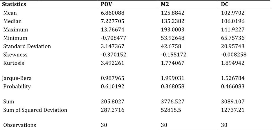
Descriptive Statistics: This section reports the descriptive statistics of poverty reduction and financial development. These statistics are the mean, median, minimum, maximum, standard deviation, kurtosis, skewness, sum, sum squared deviation and number of observations. Table 1 shows these statistics. From Table 1, we can observe that all the variables have positive average values (i.e. mean and median). This is normal considering the variables involved. In addition, the variables have minimal deviations from their means. The variables are negatively skewed as per the skewness statistics. The variables are, however, normally distributed. This shows that the skewness in the variables may not be significant. The minimum and maximum poverty recorded during the study period are -0.709% and 7.228%, respectively. Recall that POV is the household final consumption expenditure per capita growth, which means that China’s per capita household consumption has seen periods of decline (i.e. between 1988 and 1990). Interestingly, the financial sector has experienced positive growth during this period, albeit slow.
Table 1: Descriptive Statistics
Statistics POV M2 DC
Mean 6.860088 125.8842 102.9702
Median 7.227705 135.2382 106.0196
Maximum 13.76674 193.0003 141.9227
Minimum -0.708477 53.92648 65.75736
Standard Deviation 3.147367 42.6758 20.95743
Skewness -0.370152 -0.155172 -0.008258
Kurtosis 3.492261 1.774067 1.894942
Jarque-Bera 0.987965 1.999031 1.526784
Probability 0.610192 0.368058 0.466083
Sum 205.8027 3776.527 3089.107
Sum of Squared Deviation 287.2716 52815.5 12737.21
Observations 30 30 30
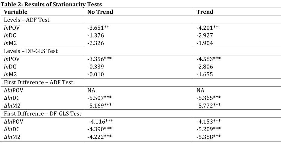
Results of Stationarity Tests: To assess the causal link between poverty and financial development in China, we test the stationarity properties of the variables. This step is crucial in order to establish the additional lag(s) (i.e. 𝑞𝑚𝑎𝑥) to include in the augmented VAR model – which will be used to test for causality following
107
Table 2: Results of Stationarity TestsVariable No Trend Trend
Levels – ADF Test
lnPOV -3.651** -4.201**
lnDC -1.376 -2.927
lnM2 -2.326 -1.904
Levels – DF-GLS Test
lnPOV -3.356*** -4.583***
lnDC -0.339 -2.806
lnM2 -0.010 -1.655
First Difference – ADF Test
∆lnPOV NA NA
∆lnDC -5.507*** -5.365***
∆lnM2 -5.169*** -5.772***
First Difference – DF-GLS Test
∆lnPOV -4.116*** -4.153***
∆lnDC -4.390*** -5.209***
∆lnM2 -4.222*** -5.388***
Notes:
1) ** and *** denote, respectively, 5% and 1% levels of significance.
2) Critical values for Dickey-Fuller GLS test are based on Elliot, Rothenberg, and Stock (1996, Table 1). 3) ∆ denotes first difference operator.
4) lnPOV = natural log of household final consumption expenditure per capita growth (annual %), lnDC = natural log of domestic private sector credit by banks (% of GDP), and lnM2 = natural log of money supply (M2) as % of GDP.
5) NA denotes non-applicable.
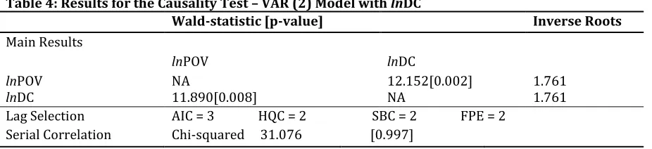
Lag Selection, Model Diagnostics, and the Results for Causality Testing: The next step in the Toda-Yamamoto causality testing is to choose the appropriate lag length. In this study, we choose the lag length based on the AIC, the Schwartz information criterion (SIC), the Hannan-Quinn criterion (HQC), and the Final prediction error (FPE). The optimal lag selected in our analysis is 2 (see Tables 3 and 4). Hence, our VAR model contains2 lags. Apart from choosing the appropriate lags, the best model must be free of serial correlation and be structurally stable. To this end, we test for structural stability and serial correlation. These results are presented in Tables 3 and 4. The inverses of the roots of the characteristic equations are higher than one in all the cases (see Tables 3 and 4), indicating that our model is structurally stable. Also, the cumulative sum of recursive residual plots shown in Figures A.1 and A.2 in the appendix supports this evidence. Moreover, our model has no serial correlation problems. This evidence is shown by the chi-squared statistic of 35.783 with a p-value of 0.984 for the lnPOV and lnM2 VAR (2) specification; and 31.076 and 0.997 for the lnPOV and lnDC VAR (2) specification, respectively.
Table 3: Results for the Causality Test – VAR (2) Model with lnM2
Wald-statistic [p-value] Inverse Roots
Main Results
lnPOV lnM2
lnPOV
lnM2 NA 8.105[0.023] 9.200[0.018] NA 1.148 1.776
Lag Selection AIC = 5 HQC = 2 SBC = 2 FPE = 2 Serial Correlation Chi-squared 35.783 [0.984]
108
Table 4: Results for the Causality Test – VAR (2) Model with lnDC
Wald-statistic [p-value] Inverse Roots
Main Results
lnPOV lnDC
lnPOV
lnDC NA 11.890[0.008] 12.152[0.002] NA 1.761 1.761
Lag Selection AIC = 3 HQC = 2 SBC = 2 FPE = 2 Serial Correlation Chi-squared 31.076 [0.997]
Note: NA denotes non-applicable.
As a final step, we fit a 𝑉𝐴𝑅(3) for all the models (i.e. 𝑛 = 2 and 𝑞𝑚𝑎𝑥 = 1) and perform the causality tests
between poverty and financial development. The results are reported in Tables 3 and 4. The results suggest that bidirectional causality exists between lnPOV and lnM2 at 5% level of significance, as evidence by the chi-squared statistics of 9.200 and 8.105, with corresponding p-values of 0.018 and 0.023, respectively, for the lnPOV and lnM2 specifications. Similarly, the results suggest that bidirectional causality exists between lnPOV and lnDC at 1% level of significance, as shown by the chi-squared statistics of 12.152 and 11.890, with corresponding p-values of 0.002 and 0.008, for the lnPOV and lnDC specifications. From these results, we can conclude that financial development may enhance poverty reduction, while the reverse is equally possible in the case of China. Ho and Odhiambo (2011) find partial support for this conclusion. Unlike Ho and Odhiambo (2011), our conclusion is independent of the proxy for financial development. Studies such as those of Abosedra et al. (2016), Sehrawat and Giri (2016a), Uddin et al. (2014), Inoue and Hamori (2012) have found evidence in favor of this conclusion as well. Essentially, the results documented in this study imply that financial development oriented policies may improve poverty reduction in China. The results also imply that policies designed to reduce poverty in China may end up stimulating financial development. Therefore, the various financial development and poverty reduction strategies that have been introduced in China over the past three decades were crucial to her financial development and poverty reduction as we see today.
5. Conclusion
The study assessed the causal links between poverty reduction and financial development in China for the period 1985–2014. The study used the Toda-Yamamoto causality test to overcome the consequences of pretesting bias that have featured majority of the existing studies. To measure financial development, the study employed two standard proxies, namely: the domestic private sector credit by banks to GDP, and money supply (M2) to GDP. For poverty reduction, the study employed a proxy that has been utilized in some of the existing studies, namely: the household final consumption expenditure per capita growth (annual percentage). The study finds bidirectional causality between financial development and poverty reduction, implying that the causality between these important variables is independent of the indicator of financial development. The findings of this study carry important policy implications. First, it implies that the poverty reduction policies and programmes implemented in China, may have led to further financial development in the country. Second, it also implies that the tremendous rate of poverty reduction in China may have been the consequence of the extensive financial sector reforms that have been carried out over the past decades. This means that financial sector reforms and poverty reduction programmes are more of “win-win” strategies in the case of China. Therefore policymakers in China should continue to implement robust financial sector reforms and poverty reduction strategies. The limitation of our study is that it employed a bivariate model to assess the causal links between poverty reduction and financial development. It is possible that other variables may connect the two variables. Therefore, future studies should identify the variables that may connect financial development to poverty reduction. That way, the evidence may come out clearer and enhance our understanding regarding the finance-poverty nexus.
References
109
Allen, F., Qian J. & Qian, M. (2005). China’s financial system: past, present and future, China’s Great Economic Transformation, edited by Loren Brandt and Thomas Rawski, Cambridge University Press.
Beck, T., Demirgüç-Kunt, A. & Levine, R. (2007). Finance, inequality and the poor. Journal of Economic Growth, 12(1), 27-49.
Birdsall, N. & Londono, J. (1997). Asset inequality matters: an assessment of the World Bank's approach to poverty reduction. American Economic Review, 87(2), 32-37.
Boyd, H., Levine, R. & Smith, B. D. (2001). The impact of inflation on financial sector Performance. Journal of Monetary Economics, 47(2), 221-248.
Burgess, R. & Pande, R. (2005). Do rural banks matter? Evidence from the Indian social banking experiment. American Economic Review, 95(3), 780-95.
Calderón, C. & Lin, L. (2003). The direction of causality between financial development and economic growth. Journal of Development Economics, 72, 321-334.
Callan, T., Nolan, B. & Whelan, C. T. (1993). Resources, deprivation, and the measurement of poverty. Journal of Social Policy, 22, 141-172.
Caner, M. & Kilian, L. (2001). Size distortion of tests of the null hypothesis of stationarity: Evidence and implication for the PPP debate. Journal of International Money and Finance, 20, 639-657.
Claessens, S. & Feijen, E. (2006). Financial sector development and the millennium development goals. World Bank Working Paper No. 89, World Bank, Washington, DC.
Datt, G. & Ravallion, M. (1992). Growth and distribution components of changes in poverty measures. Journal of Development Economics, 38(3), 275-295.
Ding, Z., Tan, L. & Zhao, J. (2011). The effect of rural financial development on poverty reduction. Issues in Agricultural Economy, 2(11), 1-13.
Dollar, D. & Kraay, A. (2002). Growth is good for the poor. Journal of Economic Growth, 7(3), 195-225.
Elliot, G., Rothenberg, T. & Stock, J. (1996). Efficient tests for an autoregressive unit root. Econometrica, 64, 813-836
Galbraith, J. (1958). The affluent society. Boston: Houghton-Mifflin.
Geda, A., Shimeles, A. & Zerfu, D. (2006). Finance and poverty in Ethiopia, UNU-WIDER Research Paper No. 2006/51, United Nations University, Helsinki, Finland.
Granger, C. W. J. (1969). Investigating causal relations by econometric models and cross-spectral methods. Econometrica, 37(3), 424-438.
Hamori, S. & Hashiguchi, Y. (2012). The effect of financial deepening on inequality: Some international evidence. Journal of Asian Economics, 23(4), 353-359.
Hao, C. (2006). Development of financial intermediation and economic growth: the Chinese experience. China Economic Review, 17, 347-362.
Hasan, I. & Zhou, M. (2006). Financial sector development and growth: the Chinese Experience, UNU-WIDER Research Paper No. 2006/85, United Nations University, Helsinki, Finland.
He, Z. & Maekawa, K. (1999). On spurious Granger causality. Economic Letters, 73(3), 307-313.
Ho, S. Y. & Odhiambo, M. N. (2011). Finance and poverty reduction in China: an empirical investigation. International of Business and Economic Research Journal, 10, 103-114.
Honohan, P. (2004). Financial development, growth and poverty: How close are the links, in C. Goodhart (ed.), Financial Development and Economic Growth: Explaining the Links, Busingstoke: Palgrave Macmillan.
Hsueh, S. J., Hu, Y. H. & Tu, C. H. (2013). Economic growth and financial development in Asian countries: a bootstrap panel Granger causality analysis. Economic Modeling, 32, 294-301.
Husain, I. (2004). Financial sector reforms and pro-poor growth: Case study of Pakistan, Presidential Address at the Annual General Meeting of the Institute of Bankers Pakistan, Karachi, 21st February, 2004. Inoue, T. & Hamori, S. (2012). How has financial deepening affected poverty reduction in India: Empirical
analysis using state-level panel data. Applied Financial Economics, 22(5), 395-403.
Jalilian, H. & Kirkpatrick, C. (2002). Financial development and poverty reduction in developing countries. International Journal of Finance and Economics, 7(2), 97-108.
Jalilian, H. & Kirkpatrick, C. (2005). Does financial development contribute to poverty reduction? Journal of Development Studies, 41(4), 636-656.
110
Levine, R., Loayza, N. & Beck, T. (2000). Financial intermediation and growth: causality and causes. Journal of Monetary Economics, 46(1), 31-77.
Lin, J. Y., Sun, X. & Wu, H. X. (2015). Banking structure and industrial growth: Evidence from China. Journal of Banking and Finance, 58, 131-143.
Lin, J. Y. (1992). Rural Reforms and Agricultural Growth in China. American Economic Review, 82, 34-51. Mack, J. & Lansley, S. (1985). Poor Britain. London: Allen & Unwin Limited.
Mood, C. & Jonsson, J. O. (2016). The social consequences of poverty: an empirical test on longitudinal data. Social Indicators Research, 127(2), 633-652.
Park, A., Ren, C. & Wang, S. (2004). Micro-finance, poverty alleviation, and financial reform in China. Rural Finance and credit infrastructure in China, OECD, 256-270.
Quartey, P. (2005). Financial sector development, savings mobilization and poverty reduction in Ghana, UNU-WIDER Research Paper No. 2005/71, United Nations University, Helsinki, Finland.
Ravallion, M. & Datt, G. (2002). Why has economic growth been more pro-poor in some states of India than others? Journal of Development Economics, 68(2), 381-400.
Schwert, W. (1986). Test for unit roots: a Monte Carlo investigation. Journal of Business and Economic Statistics, 7, 147-159.
Seetanah, B. (2008). Financial development and economic growth: An ARDL approach for the case of the small island state of Mauritius. Applied Economics Letters, 15, 809-813.
Sehrawat, M. & Giri, A. K. (2016a). Financial development and poverty reduction in India: an empirical investigation. International Journal of Social Economics, 43(2), 106-122.
Sehrawat, M. & Giri, A. K. (2016b). Financial development and poverty reduction: panel data analysis of South Asian countries. International Journal of Social Economics, 43(4), 400-416.
Sen, A. (1983). Poor, relatively speaking. Oxford Economic Papers, 35, 153-169.
Siddiki, J. U. (2002). Trade and financial liberalization and endogenous growth in Bangladesh. International Economic Journal, 16(3), 23-37
Stiglitz, J. (1998). The role of the state in financial markets, Proceedings of the World Bank Annual Conference on Development Economic, 19-52.
Takumah, W. & Iyke, B. N. (2017). The Links between economic growth and tax revenue in Ghana: an empirical investigation. International Journal of Sustainable Economy, 9(1), 34-55.
Toda, H. Y. & Yamamoto, T. (1995). Statistical inference in vector autoregressions with possibly integrated processes. Journal of Econometrics, 66, 225-250.
Turner, G., Tan, N. & Sadeghian, D. (2012). The Chinese banking system, Reserve Bank of Australia Bulletin, September, 53-64.
Uddin, G. S., Shahbaz, M., Arouri, M. & Teulon, F. (2014). Financial development and poverty reduction nexus: A cointegration and causality analysis in Bangladesh. Economic Modelling, 36, 405-412.
United Nations Development Programme. (2008). China Human Development Report. 2007-2008: Basic public services benefiting 1.3 billion Chinese people. United Nations Development Programme. World Bank. (2001). World Development Report 2000/2001, Oxford University Press, New York.
Wang, S., Li, Z. & Ren, Y. (2004). The 8-7 National Poverty Reduction Program in China – The National Strategy and Its Impact. Washington, DC: World Bank.
Wen, T., Ran, G. & Xiong, D. (2005). Financial development and the income growth of farmer in China. Economic Research Journal, 5(9).
World Bank. (1990). World Development Report 1990: Poverty, Oxford University Press, New York.
World Bank. (1995). Bangladesh: From Counting the Poor to Making the Poor Count. Poverty Reduction and Economic Management Network, South Asia Division. World Bank, Washington.
World Bank. (2009). From poor areas to poor people: China’s evolving poverty reduction Agenda. An Assessment of Poverty and Inequality in China. The World Bank, East Asia and Pacific Region. World Bank. (2014). Global Financial Development Report 2014. [Online] Available at <
http://worldbank.org/financialdevelopment >, accessed on 1 July 2016.
World Development Indicators. (2016). [Online] Available at <http://data.worldbank.org/products/wdi >, accessed on 6 July 2016.
Yamada, H. (1998). A note on the causality between exports and productivity: an empirical reexamination. Economics Letters, 61, 111-4.
111
APPENDIXFigure A.1: The cumulative sum of recursive residual plots of lnPOV and lnM2
OLS-CUSUM of equation lnpov
Time
E
m
p
ir
ica
l
fl
u
ct
u
a
ti
o
n
p
ro
ce
ss
0.0
0.2
0.4
0.6
0.8
1.0
-1
.0
0
.0
1
.0
OLS-CUSUM of equation lnm2
Time
E
m
p
ir
ica
l
fl
u
ct
u
a
ti
o
n
p
ro
ce
ss
0.0
0.2
0.4
0.6
0.8
1.0
-1
.0
0
.0
1
112
Figure A.2: The cumulative sum of recursive residual plots of lnPOV and lnDC