Computation of a Minimum Average Distance Tree on Permutation Graphs

Vol. 2, No. 1, 2012, 74-85

ISSN: 2279-087X (P), 2279-0888(online) Published on 18 December 2012

www.researchmathsci.org

74

Annals of

Computation of a Minimum Average Distance Tree on

Permutation Graphs*

Biswanath Jana1

and Sukumar Mondal2

1_{Department of Applied Mathematics with Oceanology and Computer Programming,} Vidyasagar University, Midnapore - 721 102, India.

2_{Department of Mathematics, Raja N. L. Khan Women's College, Gope Palace,} Paschim Medinipur - 721 102, India.

e-mail:[email protected]; [email protected]

Received 1 December 2012; accepted 17 December 2012

Abstract. The average distance

µ

( )G of a finite graph G= ( , )V E is the average of the distances over all unordered pairs of vertices. A minimum average distance spanning tree of

G

is a spanning tree of

G

with minimum average distance. Such a tree is sometimes referred to as a minimum routing cost spanning tree. In this paper, we present an efficient algorithm to compute a minimum average distance spanning tree on permutation graphs in

O n

( )

2 time, where n is the number of vertices of the graph.

Keywords: MAD tree, spanning tree, algorithms, complexity, permutation graphs. AMS Mathematics Subject Classifications (2010): 05C85

1. Introduction

An undirected graph G= ( , )V E with vertex set V = {1, 2, _K, }n is said to be a permutation graph iff there exists a permutation

π

= { (1), (2), , ( )}

π

π

K

π

n on {1, 2, _K, }n such that for all i j V, ∈ , ( , )i j ∈E iff

(

i j

−

)(

π

−1

( )

i

−

π

−1

( )) < 0,

j

75

given for the input graph. We assume that the permutation is stored in the array ( ), = 1, 2, , i i n

π

_K and the inverse permutation of

π

is stored in array 1

_{( ), = 1, 2, ,}

_{i i}

_n

π

−

K

. The array

_π

−1

_{( )}

_i

_{can be computed in O n( ) time from} the array

π

( )i . Figure 1 represents the permutation graph

G

and Figure 2 is the corresponding matching diagram of the permutation graph

G

.

Permutation graphs is a class of perfect graphs and can be used to solve many real world problems like the problem of airline routes connection with various cities such that all scheduled to be utilized at the same time of the day, the problem of shifted intervals etc.

Figure 1: A permutation graph G.

Figure 2: Matching diagram of the permutation graph G of Figure 1.

Breadth-first-search (BFS) is a strategy for searching in a graph when search is limited to essential two operations: (a) visit and inspect a node of a graph; (b) gain access to visit the nodes that neighbour the currently visited node. The BFS begins at a root node and inspect all the neighbouring nodes. Then for each of those neighbour nodes in turn, it inspects their neighbour nodes which were unvisited, and so on. BFS is a uniformed search method that aims to expand and examine all nodes of a graph or combination of sequences by systematically searching through every solution. In other words, it exhaustively searches the entire graph or sequence without considering the goal until it finds it.

Let

G

be a connected undirected graph, let v be a vertex of

G

and let T

be its spanning tree obtained by the BFS of

G

with the initial vertex v. An appropriate rooted tree

T v

( ) = ( , )

V E

'

⊆

G

let us call a Breadth-First-Search Tree (BFS tree, shortly) with the root v, the edges of

G

that do not appear in BFS tree let us call non-tree edges.

76

v T

∈

, i.e.,

e v( ) = max {

d v v

( , )

_i , for all

v

_i

∈

T

}

,

where

d v v

( , )

_i is the number of the edges on the shortest path between v and

v

_i. In a weighted tree

T

= ( , )

V E

' , where

|

E

'

| = | | 1

V

−

, the eccentricity e(v) of the vertex v is defined as sum of the weights of the edges from v to the vertex farthest from

v T

∈

, i.e.,

e v( ) = max {

d v v

( , )

_i , for all

v

_i

∈

T

}

,

where

d v v

( , )

_i is the sum of the weights of the edges on the shortest path between v and

v

_i.

A vertex with minimum eccentricity in the tree T is called a center of that tree T, i.e., if e s( ) = m { ( ), f in e v or all v V∈ }, then s _{is the} 1-center. It is clear that every tree has either one or two centers.

The eccentricity of a center in a tree is defined as the radius of the tree and is denoted by

ρ

( )T , i.e.,

ρ

( ) = {m

T

in e v

_{v T∈}

( )}.

The diameter of a tree T is defined as the length of the longest path in T, i.e., the maximum eccentricity is the diameter. A spanning tree with minimum diameter is defined as minimum diameter spanning tree.

The average distance

µ

( )G of a finite permutation graph G= ( , )V E is the average over all unordered pairs of vertices of the distances,

{ , } ( )

2

( ) = ( , ),

( 1) u v V G G

G d u v

n n

µ

⊂

−

∑

where

d u v

_G

( , )

denotes the distance between the vertices u and v, i.e., the length of a shortest path joining the vertices u and v.

The minimum average distance spanning tree (MAD tree, in short) of a permutation graph

G

is a spanning tree of

G

with minimum average distance.

2. Survey of the related work

In general, the problem of finding a MAD tree is NP-hard [11]. A polynomial time approximation scheme is due to [1]. Hence it is natural to ask for which restricted graph classes a MAD tree can be found in polynomial time. In [5], an algorithm is exhibited that computes a MAD tree of a given distance-hereditary graph in linear time. In [8], it is shown that a MAD tree of a given outerplanar graph can be found in polynomial time. Recently, Dahlhaus et al. [6], have design a linear time algorithm to compute a MAD tree of an interval graph which runs in O n( ) time when the left and right boundaries of the intervals are ordered. In [2], Barefoot et al., have shown that if

T is a MAD tree of a given connected graph

G

, then there exists a vertex c in T

77

computing the average distance on permutation graphs.

2.1. Applications of the problem

MAD trees, also referred to as minimum routing cost spanning trees, are of interest in the design of communication networks [11]. One is interested in designing a tree subnetwork of a given network, such that on average, one can reach every node from every other node as fast as possible.

In this paper, we have designed an

O n

( )

2 time algorithm to construct a MAD tree for a given permutation graph

G

with n vertices.

In the next section, i.e., Section

3

, we shall discuss about the construction of the tree. In subsection

3.1

, we discuss BFS tree on permutation graph. In subsection

3.2

, we discuss about the minimum diameter spanning tree. In subsection

3.3

, we develop modified spanning tree of the tree T. In Section 4, we present an algorithm to get MAD tree of the permutation graph. The time complexity is also calculated in this section.

3. Construction of the tree

3.1. Construction of BFS tree on permutation graph

It is well known that BFS is an important graph traversal technique and also BFS constructs a BFS tree. In BFS, started with vertex v, we first scan all edges incident on v and then move to an adjacent vertex w. At w we then scan all edges incident to w and move to a vertex which is adjacent of w. This process is continued till all the edges in the graph are scanned [9].

BFS tree can be constructed on general graphs in O n m( + ) time, where n

and m represent respectively the number of vertices and number of edges [17]. To construct this BFS tree on a permutation graph we consider the matching diagram. We first placed the line segment x on the zero level and all vertices adjacent to x on the first level. Next we traverse the matching diagram step by step. In first step we scan the untraversed line segment which are situated at the right side of line segments

x and in the second step we scan all untraversed line segments which are situated at the left side of the line segment x. In each iteration, we scan numbers within an interval on the top channel and scan permutation number within an interval on the bottom channel alternately in an order. Recently Mondal et al. [15], have designed an algorithm to construct a BFS tree

_{T i}

*

_{( )}

_{with root as i on trapezoid graph in O n( )} time where n is the number of vertices and Barman et al. have designed another algorithm to construct the BFS tree on a permutation graph with any vertex x as root in O n( ) time [3]. Figure 3 is the BFS tree constructed by the Algorithm PBFS [3].

3.2. Computation of minimum diameter spanning tree

Let T(1), T( (1))

π

be two BFS trees designed by Algorithm PBFS [3] of a permutation graph

G

. Let T be the minimum height tree between T(1) and

( (1))

T

π

.

78

and it is denoted by

u

*₀

→

u

₁*

→

u

*₂

→ →

_L

u

_k* , where k≤(n−1) and

u

₀* is either the vertex 1 or the vertex corresponding to

π

(1) of

G

. The vertices of the path P, i.e.,

u

_i*, i= 0, 1, 2, 3, _K, k defined as internal nodes.

We have the following terms:

The open neighbourhood of the vertex

u

_i* in the path P of

G

, denoted by *

( )

_i

N u

and defined as

N u

( ) = { : ( , )

*_i

u u u

_i*

∈

E

}

and the closed neighbourhood

* * *

[ ] = { }

_{i i}

( )

_i

N u

u

∪

N u

, where E is the edge set of the given permutation graph. Next we define level of the vertex u as the distance of u from the root i

of the BFS tree T i( ) and denote it by level(u),

u V

∈

and take the level of the root

i as

0

. The level of each vertex on BFS tree T i i V( ), ∈ can be assigned by the BFS algorithm of Chen and Das[4].

The level of each vertex of the tree T can be computed in O n( ) time.

Figure 3: BFS tree T rooted at vertex 1 of the permutation graph shown in Figure 1.

As per construction of BFS tree by the algorithm PBFS [3], we have the important result in BFS tree T.

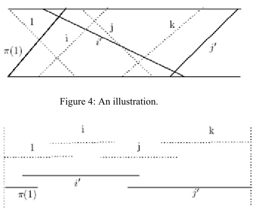
In permutation diagram, two intersecting line segments of V-type or inverted V-type defined as the scissors type line segments of permutation graphs. Figure 4 gives the illustration of scissors type line segments.

Lemma 1. Minimum number of scissors type line segments with maximum spread of the permutation diagram cover the whole region.

79 Figure 4 and Figure 5.

Firstly, if we select first dotted line segment

(1, (1))

π

−1 _{on top line. Then} we consider such line segment

( , ( ))

i

π

−1

i

_{, which is maximum spread among all} adjacent to the corresponding first line segment 1 and we marked all the line segment adjacent to 1. Next, we consider such line segment

( , ( ))

j

π

−1

j

_{which is maximum} spread among all unmarked line segment adjacent to i, continuing this process until all the line segments are covered, i.e., marked. Let this path be of the type

top→bottom→top→bottom→_K.

Similar manner to be followed from the bottom line. Then we obtain the another path of the form bottom→top→bottom→top→K. In this way whole region is covered by the both paths.

Next we consider minimum path between them which will be the shortest path to covered all the line segments. Hence, the scissors type lines segment of the permutation graph covered the whole region.

Figure 4: An illustration.

Figure 5: Region covered by the projection of minimum number of line segments.

Lemma 2. [3] Two intersecting line segments of the permutation graph of the matching diagram are assigned on the same level or adjacent levels.

Lemma 3. If u v V, ∈ and |level u( )−level v( ) |> 1 in T, then there is no edge between the vertices u and v in

G

.

Proof. If possible let |level u( )−level v( ) |> 1 but ( , )u v ∈E, i.e., u and v are directly connected. Since u and v are directly connected so by Lemma 2 either

( ) = ( )

80

assumption that |level u( )−level v( ) |> 1. Hence ( , )u v ∈E, i.e., u and v are not directly connected in

G

.

The time complexity of the algorithm PBFS is stated below.

Theorem 1. [3] The BFS tree rooted at any vertex

x V

∈

can be computed in ( )

O n time for a permutation graph containing n vertices.

Obviously, this BFS is a spanning tree.

Now, we shall prove that this spanning tree is also a minimum diameter spanning tree.

Lemma 4. The spanning tree T is a minimum diameter spanning tree.

Proof. According to the construction the BFS tree, the main path of the tree T is the longest path which is the diameter of T. The main path contains minimum number of scissors type line segments (by lemma 1). But this diameter is minimum, because T

is the minimum heighted tree between T(1) and T( (1))

π

. Also, T is a spanning

tree. Hence T is a minimum diameter spanning tree.

In next subsection, to compute the MAD tree of the permutation graph by modifying the spanning tree T.

3.3. Modification of the spanning tree T

It is observed that T is not necessarily a MAD tree. So, modification of T is necessary. We modify by following way:

Firstly compute

N u

( )

_i*

∈

G

for every internal nodes (vertices on the longest

path)

u

*_i

∈

T

. If there are any common adjacent vertices of two consecutive internal nodes of P, i.e.,

N u

( )

_i*

∩

N u

(

_i*₊₁

)

≠

φ

then by the following way we can shift them.

i) In

G

, if any common adjacent vertex w of

u

_i* and

u

_i*₊₁ exist, i.e.,

* *

1

( )

_i

(

_i

)

N u

∩

N u

₊

≠

φ

then we calculate the number of vertices to the upper side (if exist) and lower side of the internal node

u

_i* in T with

u

*_i as origin. Next calculate their difference, say,

d

₁.

ii) Again, find the number of vertices to the upper part and lower part (if exist) of the internal node

u

_i*₊₁ in T with

u

*_i+1 as origin (ignoring the vertex w). Next calculate their difference, say,

d

₂.

iii) If

d

₁

−

d

₂

≤

0

, then unaltered, i.e., w is finally adjacent of

u

_i* in T

and if

d

₁

−

d

₂

> 0

, then the adjacent vertex w of the node

u

_i* is shifted to the node *

1 i

81

Similar idea is used for pair of any two consecutive internal nodes on the main path P. Under these conditions we develop the spanning tree T and it is denoted by

'

T

. Figure 6 is the modified BFS tree

_T

' _{of the BFS tree T shown in Figure 3.}

Lemma 5. If

_T

' _{is a BFS rooted tree, then the distance}

'

( , )

T

d u v

between the

vertices u and v in T′ is given by

'

( ), if is a root,

( , ) =

( )

( ), if

* (internal node),

|

( )

( ) | 1, if be any leaf.

T

level v

u

d u v

level v

level u

u u

level v

level u

u





₋

₌





₋

₊



Proof. In the tree

_T

' _{, with u as root there exists a unique shortest path}

1 2 p 1

u

→ →

z

z

L

→

z

₋

→

v

from u to any vertex

v G

∈

, with u as parent of

1

z

and

z

_i as parent of

z

_i+1 and so on for each i= 1, 2, _K, p−2 and

z

_p−1 as parent of v. Since each vertex of this path is directly connected with the next one, hence the length of this path is p level v= ( ). Thus d u v( , )≤ p.

Next we are to show that d u v( , ) < p. If possible, let d u v( , ) = <q p. Then there exist a path

u

→ →

y

₁

y

₂

_L

→

y

_q−1

→

v

from u to any vertex

v G

∈

. As each vertex of this path is directly connected with the next one using Lemma 2,

1

( )

level y

is either

0

or 1 since level u( ) = 0. By same Lemma 2,

level y

(

_k+1

)

is either

level y

( )

_k or

level y

( ) 1

_k

+

or

level y

( ) 1

_k

−

. Thus

level y

( )

₂ is

0

or 1 or 2,

level y

( )

₃ is

0

or 1 or 2 or

3

and so on. Therefore level v( ) is

0

or 1 or 2 or...or q. This is a contradiction since level v( ) = p and

p q

>

. Hence

( , )

d u v ≤ p which implies that d u v( , ) = p, i.e., d u v( , ) =level v( ).

If _{u u=} *_{, i.e., the internal node, then as per rule of construction of BFS, there is a} shortest path

u

→ →

z

₁'

z

₂'

_L

→

v

. Here

z

₁' is at next level of _u*_, '

2

z

is at the next level of

z

₁' and so on upto v. So d(u*, z1’)= 1 =(i+1) – i, d(u*, z2 ) = d(u*, z1 ) + d(z1 , z2 ) = 1 + 1 = 2 = (i + 2) – i. If d(u*, zk ) = k = (i + k) – i, then

* ' * ' ' '

1 1

( , ) = ( , )

_{k k}

( , ) =

_{k k}

1 = (

1)

d u z

₊

d u z

+

d z z

₊

k

+

i k

+ + −

i

.

When u is any leaf, then there is a path from u to v via the parent of u. If ( ) =

level u i, then level parent u( ( )) =i−1 and parent u( ) is an internal node (as per construction of BFS rooted as 1 or

π

(1)).

Therefore

( , ) = ( , ( )) ( ( ), ) =1 ( ) ( ( ))

82

Figure 6: Modified BFS tree T of the tree T shown in Figure 3.

4. Algorithm and its complexity

In this section, we present an efficient algorithm to construct MAD tree for a given permutation graph. Also, the correctness of the algorithm and its time complexity are presented here.

Algorithm PMAD-TREE

Input: A permutation graph G= ( , )V E with its permutation representation , ( ); = 1, 2, ,

i

π

i i _K n.

Output: MAD tree

T

'and average distance

µ

( )T′ .

Step 1: Compute the minimum diameter spanning tree T //Section

3.2

// and calculate

level u

( ) = ( , ), = 1 o (1).

d u u u

* *

r

π

Step 2: Compute

N u

( )

_i*

∈

G

for all

u

*_i

∈

T

, and

k

= height of the tree T= highest level.

Step 3: //Modification of the tree T//

Compute common vertices, if any, of two consecutive internal nodes

u

_i* and

u

_i*₊₁

, = 0,

i

1, 2, , 1

_K

k

−

of the main path P may be shifted as

leaves to the node

u

_i*₊₁ under following conditions otherwise remains unaltered.

Step 3.1: For

i

= 0

to

k

−

1

do

If

N u

( )

_i*

∩

N u

(

_i*₊₁

) =

φ

then go to Step 3.1,

If

N u

( )

_i*

∩

N u

(

_i*₊₁

)

≠

φ

and let

w N u

∈

( )

_i*

∩

N u

(

_i*₊₁

)

then,

Step 3.1.1: Calculate the number of vertices to the upper part and lower part of the internal node

u

_i* in T with

u

_i* as origin. Next

83

Step 3.1.2: Calculate the number of vertices to the upper part and lower part of the internal node

u

_i*₊₁ with it as origin (ignoring the vertex w). Next calculate their difference,

d

₂.

Step 3.1.3: If

d

₁

−

d

₂

≤

0

, then unaltered and if

d

₁

−

d

₂

> 0

, then the adjacent vertex w of the internal node

u

_i* is shifted to the internal node

u

*_i+1.

Step 3.2: Set

_T

' _{as modified spanning tree of T on permutation graph}

_G

_.

Step 4: Calculate _'

( ), if is a root,

( , ) =

( )

( ), if

* (internal node),

|

( )

( ) | 1, if be any leaf.

T

level v

u

d u v

level v

level u

u u

level v

level u

u





₋

₌





₋

₊



and ' _{{ , } ( )} ' '

2

( ) =

( , )

(

1)

u v V T T

T

d u v

n n

µ

_⊂

−

∑

.

end PMAD-TREE.

4.1. Illustration of the algorithm

In Figure 3, which is the spanning tree of the permutation graph

G

,

u

_i*

= 1

and *

1

= 7

i

u

₊ are two consecutive nodes. 2 and 4 are the common adjacent of the vertices

u

_i*

= 1

and

u

_i*₊₁

= 7

, i.e., w∈{2, 4}. Taking the vertex 1 as origin, the number of vertices to the upper side of 1 is

0

and the number of vertices to the lower side of 1 is

7

. Hence their difference is

d

₁

= 7 0 = 7

−

.

Again taking the vertex

7

as origin, the number of vertices to the upper side of

7

is

3

(ignoring the vertices 2 and 4) and the number of vertices to the lower side of

7

is

6

when the vertices 2 and 4 are adjacent with the vertex

7

. Hence their difference is

d

₂

= 6 3 = 3

−

. Therefore

d

₁

<

d

₂. So, the vertices 2 and 4 are shifted to the node

7

. Then we have the modified spanning tree

_T

'_{(Figure 6).}

Next calculate the average distance

µ

₁

( )

G

corresponding to the tree T. Again calculate average distance

µ

₂

( )

G

corresponding to the tree

_T

' _{. Here}

1

( ) = 224/66 = 3.39

G

µ

(approx.) and

µ

₂

( ) = 216/66 = 3.27

G

(approx.).

Clearly,

µ

₁

( ) >

G

µ

₂

( )

G

. Hence

T

'is the minimum average distance tree of permutation graph

G

.

Theorem 2. The tree formed by Algorithm PMAD-TREE is the MAD tree.

84

connect all other vertices directly with the internal nodes. Again, since the leaves in level difference two or more in BFS, are not adjacent so they may be connected via their parent vertex, i.e., internal nodes (Lemma 2 and Lemma 3). So to get minimum average distance one leaf may be shifted to immediate level, i.e., adjacent to just next internal node. Therefore sum of the distances among all pair vertices through the main path is minimum (Lemma 5). Again by Step

3

, we check the distances among leaves of the tree. The condition of shifting the leaves to other, if necessary, implies sum of the distances among the leaves, after modification, is minimum. Hence, sum of the distances among the vertices in tree is minimum. Therefore, the tree formed by

Algorithm PMAD-TREE is a MAD tree.

Next we describe the time complexity of the algorithm.

Theorem 3. The MAD tree of a permutation graphs

G

with n vertices, by Algorithm PMAD-TREE, can be computed in

_{O n}

_{( )}

2 _time.

Proof. Step 1 takes O n( ) time (Theorem 1). Step 2, i.e., computation of open neighbourhood of all internal nodes on the main path and add with corresponding nodes can be computed in

O n

( )

2 time. Each Step 3.1.1 and Step 3.1.2 takes O n( ) time. Also Step 3.1.3 runs in O(1) time. But Step 3.1 runs

k

−

1

times, so total time complexity of Step 3.1 is

_{O n}

_{( )}

2 _{, where}

_k

_{is of O n( ). Again Step 3.2, i.e.,} modification of the tree can be computed in

_{O n}

_{( )}

2 _{time. The last step, i.e., Step 4 in} worst case, can be computed in

_{O n}

_{( )}

2 _{time. Hence, overall time complexity of our}

proposed algorithm is

_{O n}

_{( )}

2 _{time with n vertices of permutation graphs.}

REFERENCES

1. Bang Ye We, Lancia, G., Bafna, V., Chao, K. M., Ravi, R. and Chuang Yi Tang, A polynomial time approximation scheme for minimum routing cost spanning trees, SIAM Journal on Computing, 29 (1999) 761 - 778.

2. Barefoot, C. A., Entringer, R. C. and Szekely, L. A., Extremal values of distances in trees, Discrete Applied Mathematics, 80 (1997) 37 - 56.

3. Barman, S., Mondal, S. And Pal, M., An efficient algorithm to find next-to shortest path on permutation grphs, Communicated.

4. Chen, C. C. Y. and Das, S. K., Breath-first traversal of trees and integer sorting in parallel, Information Processing Letters, 41 (1992) 39 - 49.

5. Dahlhaus, E., Dankelmann, P., Goddard, W. and Swart, H. C., MAD trees and distance-hereditary graphs, Discrete Applied Mathematics, 131 (2003) 151 - 167. 6. Dahlhaus, E., Dankelmann, P. and Ravi, R., A linear time algorithm to compute a MAD tree of an interval graph, Information Processing Letters, 89 (2004) 255 - 259.

7. Dankelmann, P., Computing the average distance of an interval graph, Information Processing Letters, 48 (1993) 311 - 314.

85

9. Deo, N., Graph theory with applications to engineering and computer science (Prentice Hall of India Private Limited, New Delhi, 1990).

10. Golumbic, M. C., Algorithmic graph theory and perfect graphs, Academic Press, New York, 2004.

11. Johnson, D. S.,Lenstra, J. K. and Rinnooy-Kan, A. H. G., The complexity of the network design problem, Networks, 8 (1978) 279 - 285.

12. Muller, J. H. and Spinrad, J., Incremental modular decomposition, J. ACM, 36 (1989) 1 - 19.

13. Olariu, S., Schwing, J. and Zhang, J., Optimal parallel algorithms for problems modeled by a family of intervals, IEEE Transactions on parallel and Distributed Systems, 3 (1992) 364 - 374.

14. Pnueli, A., Lempel. A. and Even, S., Transitive orientation of graphs and identification of permutation graphs, Canad. J. Math., 23 (1971) 160 - 175. 15. Mondal, S., Pal, M. and Pal, T. K., An optimal algorithm for solving all-pairs

shortest paths on trapezoid graphs, Intern. J. Comput. Engg. Sci. 3 (2002) 103-116.

16. Mondal, S., Pal, M. and Pal, T. K., An optimal algorithm to solve the all-pairs shortest paths problem on permutation graphs, Journal of Mathematics Modelling and Algorithms, 2 (2003) 57 - 65.