Volume 6(Fall 2009) Article 6
7-17-2012
Team Production Function and Player Shirking in
Major League Baseball
Michael Kodesch
Kevin Macios
Follow this and additional works at:http://commons.colgate.edu/car
Part of theLabor Economics Commons
This Article is brought to you for free and open access by the Student Work at Digital Commons @ Colgate. It has been accepted for inclusion in Colgate Academic Review by an authorized administrator of Digital Commons @ Colgate. For more information, please contactskeen@colgate.edu.
Recommended Citation
Kodesch, Michael and Macios, Kevin (2012) "Team Production Function and Player Shirking in Major League Baseball,"Colgate Academic Review: Vol. 6, Article 6.
Team Production Function and Player Shirking in Major
League Baseball
By Michael Kodesch, Class of 2010, and Kevin Macios, Class of 2010
Introduction
Major League Baseball has long been recognized as a useful tool in modeling other labor markets. Not only does the system perfectly replicate personal psyche and motivation, but few other industries record worker statistics to the extent of the MLB. In fact, members of the Society for American Baseball Research (SABR) are dedicated to producing a myriad of performance measures in an attempt to help quantify individual and team production. With these measures, various topics can be discussed within a numerical context. Baseball is also a very interesting industry due to its monopsonistic nature, where the owner has total contract control in a sea of salary-hungry players.
Despite the expansive amount of research dedicated to shirking1, researchers and econometricians have yet to reach agreement on whether this dark art exists within Major League Baseball. The issue has become the forefront of owners’ concerns with the advent of long-term contracts, largely because pay is now uncoupled with performance. In lieu of contract incentives, on-field player performance has become questionable in light of guaranteed income and security.
The first section of this paper is
dedicated to understanding the
background of shirking in a historical context. There have been four critical eras in this time frame in which
contracts have experienced systematic change, resulting in differing player attitudes towards productivity. While the owners’ preferences have remained constant through these four eras, players have received different circumstances regarding salaries, and have leveraged their performance to compensate these changes.
The second part of our analysis empirically estimates a production function across both the American and National leagues using models previously specified in conjunction 21with stipulations derived from the new baseball regime. Cross-sectional data was acquiesced from the 2007 and 2008 seasons and is used in a multiple regression analysis. We will be able to determine a reliable estimate for the production function which will assist us later in our shirking analysis. With this production function, a team could very easily appropriate a salary structure for their players given the revenue information of the firm
Finally, based on the production function, the third section of the paper will establish the marginal productivity of individual players. In particular, we will be focusing on a group that has signed multi-year contracts between the 2007 and 2008 seasons. To aid the
211Sherony says “a player shirks when his pursuit of a
statistical adequacy of our two-part model, we will also include the analysis of two additional groups, one-year contract players and players that are in the second year of a contract to control for any stochastic variance in player performance.
Baseball contains significant differences from other production processes, and there must be some caution when translating results. However, sports labor markets at the least “can be seen as a laboratory for
observing whether economic
propositions at least have a chance of being true” (Kahn 2000). In this light, we can make some important inferences in regards to long-term contracts and their subsequent effect on performance in a larger context.
I. Background
The first era of Major League baseball (1865-1921) was most notably a transition from an amateur to a professional sport. There was little structure within the league in terms of player salaries, where baseball was mostly a part-time affair. Due to the loose nature of the system, a form of
shirking was practiced termed
“hippodroming,” describing payments made from gamblers to players to assure results in high-stakes games. The most infamous incident of hippodroming was the Black Sox scandal of 1919, in which eight players were banned from baseball for taking part in throwing the World Series. The major issue within the scandal stemmed from poor relations between the monopsonistic owner and the players. In order to exploit an
incentive within these player’s contracts, the owner physically controlled player output by directly impeding player production, resulting in resentment and distrust between the two parties. This distrust has served as a strong foundation for the relations between owners and players today, and continues to act as an ingredient for the propensity to shirk.
In 2003, Glenn Knowles calculated stochastic frontier estimations for the career of Babe Ruth, which yielded some particularly interesting results. Many players shirk by becoming injured more often, allowing them to play less at the team’s expense. In Knowles’ study, total bases were used as the key output for performance; a measure that effectively takes playing time into account. After comparing the actual data to Babe Ruth’s stochastic frontier, two largely skewed terms show up in 1922 and 1925, with 1922 being the first year of Ruth’s long term contract. This contract had no incentive bonuses and consequently, Ruth’s batting average and other average statistics had dropped significantly. His behavior during both periods of lackluster execution can be directly attributed to both his on-field and off-field performance. To confirm
that shirking existed, Ruth
“acknowledged his mistakes and vowed to work hard, which he did accomplish the next season” (Knowles 2002).
The third era of baseball, from which our model was acquired, marked a period of open free agency. Starting in 1973, the reserve clause was nearly dropped as players who performed one season without a signed contract would be eligible to sell their services to the highest bidder. Salaries sky-rocketed giving birth to a contract that would secure a player on a team for some time: the long-term contract. In 2001, of all players who were eligible for salary arbitration, “62.9 percent had multi-year
contracts. Furthermore, when
considering the twenty-five players with one year contracts who also had option years as part of their deal, only 32
percent of experienced players had one-year contracts” (Sherony 2002). With a large prevalence of long-term deals in mind, owners became haunted with the pretense of shirking within their firm.
Anthony Krautmann conducted a study in 1990 measuring the marginal productivity of players scattered throughout history against a stochastic interval based on means, standard errors, and extrema analyses. By using a player’s slugging average, Krautmann was unable to reject the null hypothesis that shirking did not exist and instead credited any variance in performance to the stochastic nature of baseball. As noted earlier, however, shirking is also the byproduct of an increased propensity to be injured, and is not reflected within the slugging
average statistic. Furthermore,
Krautmann admits this flaw citing a study that concludes “on average, every additional year remaining on a multi-year contract was associated with a 25 percent increase in number of days spent on the disabled list, as well as a significant increase in the probability that a player is injured” (Lehn 1982).
In 1997, Mark Woolway
extrapolated a different model that accounted for injury and once again put shirking on trial. Additionally, he designed his model to adjust for players that switched teams from non-contract year to contract year. After calculating a production model based on the 1993 season for team victories, he calculated the marginal products of players before and after entering a long-term contract, and found results that contradicted those of Krautmann.
While Woolway’s model takes the
consideration, there are a few significant changes found in today’s regime that must be addressed. During the Labor Strike of 1994 and 1995, player salaries once again increased tremendously, in lieu of any expectations of increased performance. The implications of shirking seem more relevant and threatening in this environment; the possible existence of which motivates the primary question in our study. Moreover, certain statistics within the game have become either more or less prominent, changing the effectiveness of Woolway’s model. Finally, while Woolway only included a list of long-term contract players in their first year, it is equally important to analyze players in different situations to touch base with regression towards the mean.
II.Empirical Estimate of Major League Baseball’s Production Function
Using Woolway’s model as a guide, we will run a cross-sectional regression using data from the 2007 and 2008 seasons. Accordingly, we will use the Cobb-Douglas functional form as it is very straightforward in reporting relative factor shares and returns to scale. We will also be using the same dependent variable, team win percentage (W%), as it ultimately explains a team’s productivity and success. “Other considerations play a part in determining team revenue, such as stadium amenities, player popularity, and geographic location, but the major element in long run profitability of a team is success on the playing field” (Woolway 1997). It is important to note that using team wins is analogous to
using team win percentage as all teams play the same amount of games during the regular season.
The inputs that determine team win percentage fall under three categories: offense, defense, and pitching. In simple terms, a team must score runs to win games (offense), while limiting runs scored by the opposing team (defense and pitching). Speed has become increasingly important in the game of baseball, as it affects both stolen bases for offense as well as a player’s range in the field.
Sabermetricians have come up with a seemingly endless list of statistics that describe offense; however, we will focus on three statistics that encompass everything that an offense can produce. The first two statistics fall under hitting. Hitting can be broken down into two sub-skills: hitting to get on base, and hitting for power. Past models had used batting average, but we find this to be incomplete, as walks and hit-by-pitches factor into getting on base, and ultimately assist teams in scoring runs. For this reason, we have incorporated the statistic On-Base Percentage (OBP) in our model. OBP is calculated the following way:
OBP = [hits + walks + hit-by-pitches] / [at-bats + walks + sacrifice flies + hit-by-pitches]
of bases earned from hits by the total number of at bats, which effectively realizes singles, doubles, triples, and home runs. Despite its illusive name, it is important to note that a player can theoretically achieve a slugging percentage greater than one, two or three for that matter, though this is not commonly seen over the course of a season. After running the full regression with offense, defense, and pitching, we discovered a large deal of variance inflation between SP and OBP. Looking closer, the two statistics have become increasingly correlated since the 1993 season model. Because it is important to include both types of hitting as both types of hitters exist, SABR has recently come up with a statistic that combines these two categories, called On-Base plus Slugging Percentage (OPS). This value is calculated simply by adding OBP and SP. The third and last component of offense is stolen bases (SB), as thieveries increase the chances to move runners into scoring position, and subsequently increasing the chance to score runs.
The second major input to calculate team win percentage is the efficacy of a team’s pitching staff. As the efficiency of pitching increases, less runs are scored giving the team a better chance of victory. In this respect, we are in full agreement with Woolway that Earned Run Average (ERA) is the best statistic to incorporate. Earned run average is calculated on a nine inning basis by multiplying the total amount of earned runs by nine and then dividing by the total innings pitched. Earned runs are scored runs that did not involve the complacency of fielding, but were scored on what statisticians identify as hits.
Runs that are the result of a defensive mishap are recorded as an error for a player on defense rather than a hit, and are measured within the statistic called unearned runs (UER). In past models, the ratio of strikes to walks was used as
the key indicator of pitching
performance. However, some of today’s best pitchers have low strike out totals but are extremely effective on the mound by forcing batters to ground out and fly out. This would not show up within the context of strikes to walks, whereas ERA can consistently measure the adequacy of a pitcher.
Woolway designates defense as the final component in determining team production. In past models, fielding percentage and total chances were found to be statistically insignificant in a production model. In light of this insignificance, Woolway used the UER
statistic aforementioned which
Our last difference between the model of Woolway and our theoretical model involves the use of a dummy variable separating differences between the American and National Leagues. Dummy variables should be included in a model where the same inputs produce a different output due to qualitative differences. However, since there is very little interleague play, AL and NL win percentages should both be centered around mean .500. Since the standard deviations and means of win percentage
of the different leagues are
approximately the same, we have left out the dummy variable from our model. On a separate note, Woolway’s dummy variable came out to be insignificant at the 10% significance level, supporting our claim.
By removing the logarithms from our four variables, W%, OPS, SB, and ERA, we can prepare our variables for
multiple-regression analysis.
Additionally, we followed Woolway’s model by indexing each of these logged variables in order to standardize the differences in measures. In order to do this, we divided each of the categories by their respective American League and National League averages in attempt to enable inference. We now have the following equation and regression result:
*Data is based off of MLB data from ESPN.com and MLB.com
Parameter Estimates
Variable D F
Parameter Estimate
Standard
Error t Value Pr > |t|
Variance Inflation
Intercep t
1 1.57140 0.34417 4.57 <.0001 0
ops 1 2.54743 0.26828 9.50 <.0001 1.03278
sb 1 12.03826 4.26057 2.83 0.0065 1.03889
The data that we used is from reliable baseball reporting websites. Every team and year is counted as a separate observation, so that we ended up with 60 sets of different W%, ERA, SB, and OPS. As for win percentage, because the teams play the same amount of games and the competitive balance is theoretically equal between all teams, the histogram for win percentage is approximately normal.
It is extremely important that the model is well specified in order to make consistent and unbiased inferences. The second part of our analysis involves using the production function to calculate marginal productivities of several groups of players. If the model above is wrongly specified, then any inferences we try to draw from our final product would be meaningless. For this reason, several tests and graphs were constructed to ensure the reliability of our model.
As the table shows, all of the variables used are statistically significant at the 1% alpha level. Additionally, the variance inflation levels are relatively low indicating the absence of significant multi-collinearity. After reviewing graphs of the residuals against different variables, there is no evidence of heterogeneity within the data [Figures 6 and 12]. Additionally, since the residuals are uncorrelated with the independent variables, there is no evidence of omitted variables bias. Although it is warranted to be cautious, as the outcome of a game is determined by many factors. With the exception of a few outliers, there exists no pattern suggesting that the variables require a different functional form. Our adjusted R2 value was equal to .8042, which can be interpreted as a relatively
strong correlation between the explained and explanatory variables.
In order to test whether non-linearities had been excluded from our model, we performed a regression specification error test (RESET) [Figure 7]. With numerator degrees of freedom equaling 4 and denominator degrees of freedom equaling 53, we regressed our dependent variable over squared and cubed terms of our predicted y-hats from the original production function. With a critical value of approximately 2.58 at a 5% significance level, we calculated an F-value of .94 and a corresponding p-F-value of .3985. With this information, we cannot reject the null hypothesis that the coefficients of the non-linear possibilities equal zero. This means that the model does not need any non-linearities, as the current definition is adequate.
Finally, to test whether the assumption of homoskedasticity holds, we performed a Breusch-Pagan test [Figure 8] as well as a White test [Figure 9]. The null hypothesis of both tests posits that the model is homoskedastic. With degrees freedom 4 and significance level .05, we fail to reject at a critical value below 9.49. After completing the tests, we received Chi-squared values of 3.55 and 1.02 for the BP and White tests respectively. With this information, we fail to reject the null hypothesis, and our model can be considered homoskedastic.
III. Model for Calculating Marginal Productivity of Major League Baseball Players
Our first reaction to analyzing a change in one year from the next was to use a two period panel. This is almost always the most appropriate method in understanding policy change. However, there are several problems within the realm of baseball that made this approach obsolete. First, there are only 40 to 50 long term contracts granted per year. Two period panel models work best when the amount of observations is great enough to outweigh any outliers. Also, many players sign long term contracts with a different team from their non-contract year, creating irregularities in terms of what to use for the difference in the dependent variable. The final predicament we ran into when using this model was finding that the residuals were correlated with our explanatory variables, rendering the model useless. For this reason, we can account for all of the problems in the two period panel model with our current strategy using a production function and marginal analysis.
Once there is a working model able to predict a team’s win total, it can be applied to the final step in deciding whether or not players shirk. The team production function model is crucial to this second model as player productivity will be determined with respect to the player’s contribution to his team; after all, it is the team that should be most concerned with whether or not a player shirks. A player’s marginal productivity will essentially be determined by how many wins that player added or subtracted from a team. Presumably a
player who shirks will contribute less wins in the year preceding the signing of his new multi-year contract than he did in the year before.
In order to account for all variation and to safely be able to conclude that shirking either does or does not exist, three groups of players were put through the model. All three groups consisted of 43 players; 26 position players and 17 pitchers. The first group is the 43 players who signed multi-year contracts between the 2007 and 2008 seasons. This is where our sample size of 43 comes from. The second group is a random group of 43 players who signed one year contracts between the 2007 and 2008 seasons. The third and final group is a random sample of 43 players who signed multi-year contracts between the 2006 and 2007 seasons and therefore had not yet completed their contracts entering the 2008 season. In order to select these random groups, two separate lists were compiled including all of the one-year contract players for one list, and all of the second year long term contract players on the other. After dividing the pitchers from the position players, random numbers were assigned to each name. Finally, to pick these players for analysis, 17 and 26 random numbers were generated for pitchers and hitters respectively to create the two extra data sets.
or if their seasons were simply products of the stochastic nature of baseball. By including these control groups we can compare the marginal productivities of the players who signed multi-year contracts to the marginal productivities of other players in major league baseball. In theory, these control players have extra incentive to play better as they are presumably trying to earn multi-year contracts for a guaranteed salary.
In order to consider the marginal productivity model accurate, a few assumptions must be made. First, we assume ceteris paribus alongside of the multi-year contract. While the base year is held constant in our model to account for players that switch teams, there are a few assumptions that must be made to allow for ceteris paribus. We must assume that a player’s performance for moving from a hitter-friendly stadium to a pitcher-friendly stadium, or vice-versa, is negligible. Additionally, players who change teams moving into a more or less productive lineup, bolstering or weakening said player’s statistics must also be assumed insignificant. It should also be noted that each player’s ability may have waned with one additional year of age or increased with an additional year of experience. Later in our paper we will consider this factor by breaking up players and their respective results into three sets of ages to analyze any disparities in marginal product.
The first step in calculating a player’s marginal productivity is to compare the team’s 2007 predicted win total to the model-predicted win total of the same team without the player’s 2007 stats. The difference between these two win totals
is the player’s marginal productivity for the 2007 season. A positive number indicates that the player won that many more games for the team in 2007 than the team would have won without him. Likewise, a negative number indicates that the player’s performance was sub-par and cost his team that many wins in 2007.
The next step is to calculate each player’s marginal productivity for the 2008 season. This is where we need to designate a base year so that everything other than the player’s change in performance can be held constant. By taking the team’s 2007 performance minus the player’s stats from 2007, and adding the player’s 2008 stats, the new set of team statistics represents what the team would have done if they had had the 2008 version of the player in question on the 2007 team. Again, by comparing the model-predicted win total of this new set of stats to the model-predicted win total of the 2007 team without the 2007 (or the 2008) player, the resulting number represents the player’s 2008 marginal productivity.
Now that we have the marginal productivities of each player from 2007 and 2008, we can look into shirking. The difference between the two marginal productivities represents the change in a player’s productivity between the 2007 season and the 2008 season. A positive number indicates that the player produced that many more wins in 2008 than he did in 2007. A negative number indicates that the player produced that many fewer wins in 2008 than he did in 2007.
and changes in marginal productivities were calculated accordingly [Figure 11]. The change in marginal productivity
from 2007 to 2008 for the three main samples of players can be summarized as follows:
The results obtained from the marginal productivity model appear to suggest that shirking does indeed exist among players who sign multi-year contracts. Both pitchers and position players who signed long-term contracts between the 2007 and 2008 seasons saw their marginal productivities decline on average. The two other groups – players who signed one-year contracts for 2008 and players who were in the midst of a multi-year contract – showed on average an increase in marginal productivity from 2007 to 2008. The fact that these numbers are small implies regression to the mean, and the variance from year to year for a player still solicits evidence of stochastic production.
In order to make inferences from these results, we will now test these sets to consider sample size and deviation from the mean. Since our data strictly relies on a change in marginal productivity, we can apply a one-tailed t-test at a 5% significance level to see whether performance for each group had
declined. The test for all players who signed multi-year contracts between the 2007 and 2008 seasons resulted in a tstatistic of 1.75 and a critical value of -1.684. The null hypothesis that the players’ marginal productivities did not decline after signing their new multi-year contracts is rejected. For pitchers alone the t-statistic is -2.038 with a critical value of -1.753, while the t-statistic for hitters is 5.469 with critical value of -1.711. In both instances, the null hypothesis can once again be rejected. At this point in his research, Woolway concluded that shirking existed in the 1993 season. However, we must also test the other sets before making a generalized conclusion.
For players who signed one-year contracts prior to the 2008 season, the t-tests failed to reject the null hypothesis that their marginal productivities had declined. The same can be said for players in the second year of a long-term contract, where the t-tests lacked evidence to find declines in marginal
Group Pitchers Position
Players
Combined
’08 Multi-year contracts
-0.84 -1.34 -1.14
’08 One-year contracts
0.07 0.34 0.23
’07 Multi-year contracts
productivity [Figure 10]. Using all three pieces of knowledge, we have come to the conclusion that shirking exists the year after a player signs a long term contract. While a one game reduction in wins may seem insignificant for a 162 game season, we speculate that it is noteworthy in at least two specific historical contexts. “The first Dodger team to finish last in eighty-seven years had acquired five 1991 [long-term contract signers]. Similarly, the Mets team that collapsed in 1993 had acquired
three 1992 [long-term contract signers]” (Vrooman 1996).
Woolway continues his study by addressing age as a possible component in productivity differences from year to year. We decided to break down age into slightly different categories than that of previous models, as 28-32 is considered a player’s prime in the new era of baseball. After computing the marginal differences in year to year performance, we came up
with the following results:
Pitchers
Group 27 and under 28-32 33 and above
’08 Multi-year contracts -1.05 -0.97 0.28
’08 One-year contracts 0.00 0.45 -0.98
’07 Multi-year contracts 0.77 0.45 1.00
Position players
Group 27 and under 28-32 33 and above
’08 Multi-year contracts -1.19 -1.25 -2.15
’08 One-year contracts 0.15 0.42 0.65
Combined
Group 27 and under 28-32 33 and above
’08 Multi-year contracts -1.14 -1.14 -1.18
’08 One-year contracts 0.09 0.43 0.10
’07 Multi-year contracts 0.73 0.17 0.66
Players who signed multi-year contracts between the 2007 and 2008 seasons saw their marginal productivities decline across all age groups except for one: pitchers ages 33 and above. This sample of players consists of only two pitchers, Troy Percival and Mariano Rivera, both 38 years old. Percival experienced a decline in marginal productivity of
roughly one game but Rivera’s
productivity increased by over a game and a half. With a sample size this small, a t-test to reveal any existence of shirking is inconclusive.
One-year contract players and second year contract players saw positive changes in marginal productivity over all age ranges and positions except for one. In this case, pitchers ages 33 and over saw their marginal productivities decline by almost one game. It is possible that this is another anomaly, especially since the set once again only contains two pitchers. However, it is more likely that these players are experiencing a natural decline in productivity as they get older, particularly Tom Glavine who was 43 years old in 2008. The fact that these two pitchers only received one-year contracts may be indicative of their declining skill set. Overall, age does not appear to be as much of a factor in player marginal productivity as signing a multi-year
contract is. Essentially, shirking spans all age groups within players who are in the first year of a multi-year contract. Regardless of age, other players are subject to the stochastic nature of baseball.
IV. Conclusion
Major League Baseball offers a unique opportunity to study the behavior of buyers and sellers in a market with supporting statistics for their respective movements. As economists, we can use this lucrative setting to extrapolate both sociological and psychological patterns that influence similar systems. In our paper, we have specified a statistically adequate relationship to effectively model team victories using the explanatory variables OPS, SB, and ERA. The combination of these statistics fully encompasses the offense, defense, and pitching of a major league baseball team and a player’s marginal product can be ascertained through the clever use of the model.
many owners’ arguments that vouch for one-year contracts to protect them from the evident shirking associated with long-term contracting. As Woolway recommends, a regime of one-year contracts would create performance incentive rather than performance disincentive.
Owners should concern
themselves with the aggregate effect that these findings can potentially have on a team. One player shirking on a team costing, on average, one win may not make a difference. Then again, it might make a huge difference when you consider that the 2007 New York Mets
finished one game behind the
Philadelphia Phillies for the NL East title and subsequently missed the playoffs. Also consider a team that has five players on their team signed to multi-year contracts. If those five players combine to cost their team five wins it could have drastic effects. Consider the 2008 Phillies who won 92 games and went on to win
the World Series. If the Phillies had lost five additional games they would have missed the playoffs all together.
The next question to ask is how these findings can be related to other job and labor systems. It is possible and even likely that other industries granting similar job security may be prone to the same negative effects. Institutions that utilize methods such as seniority rule or tenure may be making themselves vulnerable to similar disincentive effects. We cannot easily assume a professor would act differently to tenure than a baseball player would to a guaranteed long-term contract. Yet, just as it may take an aggregate of several shirking players to have a substantial impact on a team, a combination of several shirking professors may have a substantial impact on a University. With this note, we encourage managers within comparable labor systems to conduct similar research
Appendix:
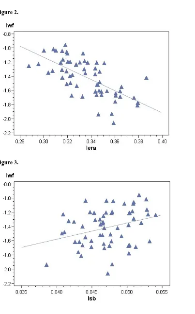
Figure 1. 2007-2008 Team Win Percentage vs. Team OPS Figure 2. 2007-2008 Team Win Percentage vs. Team ERA Figure 3. 2007-2008 Team Win Percentage vs. Team SB Figure 4. 2007-2008 Team Win Percentage vs. Team UER Figure 5. 1993 Team Win Percentage vs. Team UER Figure 6. 2007-2008 Residual vs. Predicted Win Percentage Figure 7. Results of a RESET test
Figure 8. Results of a Breusch-Pagan Test Figure 9. Results of a White test
Figure 10. T-test Results for Marginal Productivity
Figure 11. Marginal Productivity listed by player, position and contract Figure 12. Residuals vs. Independent Variables
Figure 2.
Figure 4.
Figure 6.
Figure 7.
Test 1 Results for Dependent Variable lwf
Source DF
Mean
Square F Value Pr > F
Numerator 2 0.01233 0.94 0.3985
Denominator 54 0.01317
Figure 8.
Root MSE 0.01763 R-Square 0.0592
Dependent Mean 0.01227 Adj R-Sq 0.0088
Figure 9.
Root MSE 0.01786 R-Square 0.0171
Dependent Mean 0.01227 Adj R-Sq -0.0174
Coeff Var 145.56521
Figure 10.
Pitchers
Group n xbar se crit. t
’08 Multi-year contracts 43 -0.84 0.414 -1.753 -2.038
’08 One-year contracts 43 0.07 0.506 -1.753 0.136
’07 Multi-year contracts 43 0.75 0.427 -1.753 1.759
Position players
Group n xbar se crit. t
’08 Multi-year contracts 43 -1.34 0.244 -1.711 -5.469
’08 One-year contracts 43 0.34 0.317 -1.711 1.082
’07 Multi-year contracts 43 0.264 0.286 -1.711 0.923
Combined
Group n xbar se crit. t
’08 Multi-year contracts 43 -1.14 0.652 -1.684 -1.750
’08 One-year contracts 43 0.23 1.019 -1.684 0.230
Figure 11.
’08 Multi-year contracts
Pitcher Age ΔMP Hitter Age ΔMP
Manny Corpas 25 -2.26 Yadier Molina 25 0.26
James Shields 26 0.45 Miguel Cabrera 25 -1.49
Dontrelle Willis 26 -0.72 Ian Kinsler 25 1.89
Jake Peavy 26 -1.67 Brandon Phillips 26 -1.73
Johan Santana 29 2.32 Robinson Cano 25 -2.84
Rafael Soriano 28 -0.78 Troy Tulowitzki 23 -2.24
Rafael Betancourt 32 -3.56 Curtis Granderson 27 -2.16
Scott Downs 32 0.59 Ross Gload 32 -1.04
Nate Robertson 30 -3.09 Carlos Pena 29 -2.54
Carlos Silva 29 -4.14 Marco Scutaro 32 0.23
Aaron Cook 29 0.57 Matt Holliday 28 -1.10
David Riske 31 -1.78 Alex Rodriguez 32 -3.01
Scott Linebrink 31 -0.09 Andruw Jones 31 -1.50
Francisco Cordero 32 -0.21 Aaron Rowand 30 -2.98
J.C. Romero 31 -0.52 Jose Guillen 31 -1.65
Troy Percival 38 -1.00 Kazuo Matsui 32 -0.24
Mariano Rivera 38 1.56 Yorvit Torrealba 29 0.33
Khalil Greene 28 -2.56
Torii Hunter 32 -0.76
Freddy Sanchez 30 -2.03
Luis Castillo 32 -0.23
’08 One-year contracts
Pedro Feliz 32 -0.15
Geoff Jenkins 33 -1.12
Mike Lowell 34 -2.03
Jorge Posada 36 -3.30
Pitcher Age ΔMP Hitter Age ΔMP
John Danks 24 3.51 Alexi Casilla 24 0.97
Francisco Liriano 25 -2.88 Willy Taveras 27 -0.80
Fausto Carmona 25 -5.11 Miguel Cabrera 23 -1.48
Edison Volquez 25 2.70 Asdrubel Cabrera 26 -0.44
Huston Street 25 -0.35 Justin Morneau 27 0.99
Daniel Cabrera 27 0.55 Franklin Gutierrez 26 -1.28
Zack Greinke 25 1.02 Carlos Quentin 26 5.01
Joakim Soria 24 0.55 Mark Teahen 27 -1.45
Dan Wheeler 31 1.31 Delmon Young 23 0.54
Aaron Heilman 30 -2.24 Carlos Gomez 23 -0.43
Matt Belisle 28 -0.03 Omar Infante 27 0.03
Kerry Wood 31 0.21 Ty Wiggington 31 4.68
Justin Duchscherer 31 2.88 Chris Snyder 28 -1.30
Brad Lidge 32 0.95 Xavier Nady 30 -1.11
Bobby Jenks 28 0.05 Jose Castillo 28 0.23
Tom Glavine 43 -0.61 Cesar Izturis 29 -0.99
Andy Pettitte 36 -1.35 Rick Ankiel 29 0.72
’07 Multi-year contracts
Luke Scott 30 -0.41
Kevin Youkilis 30 2.50
Eric Hinske 31 1.06
Adam Everett 32 -0.74
Sean Casey 34 0.67
Gabe Kapler 34 1.05
Cliff Floyd 36 0.09
Casey Blake 35 0.79
Pitcher Age ΔMP Hitter Age ΔMP
Daisuke Matsuzaka 27 4.70 Brian McCann 24 2.68
Jeff Francis 27 -1.54 Joe Mauer 25 1.27
Brett Myers 27 0.10 Austin Kearns 27 -1.93
Matt Cain 23 -0.20 Aubrey Huff 31 2.66
Jason Marquis 29 0.37 Julio Lugo 32 -3.45
Ted Lilly 32 -0.72 J.D. Drew 32 2.12
Gil Meche 29 -0.70 Alfonso Soriano 32 -1.01
Scot Shields 32 0.88 Aramis Ramirez 29 0.12
Adam Eaton 30 1.65 Jason Michaels 31 -0.87
Vicente Padilla 30 1.22 Carlos Lee 31 -0.56
Chad Bradford 33 0.55 Juan Pierre 30 -0.84
David Weathers 38 0.13 Chase Utley 29 -0.91
Justin Speier 35 -1.51 Vernon Wells 29 1.78
Guillermo Mota 34 1.29 Akinori Iwamura 29 -0.91
Mike Mussina 39 4.26 Lyle Overbay 31 1.16
Jamie Moyer 45 2.96 Jay Payton 34 0.00
Mark DeRosa 33 1.55
Gary Matthews Jr. 33 -0.97
Craig Counsell 37 0.38
Bengie Molina 33 0.67
Rich Aurilia 36 0.96
Dave Roberts 35 -0.14
Ray Durham 36 2.54
Brian McCann 24 2.68
References
Hakes, Jahn and Chad Turner, (2007) “Pay, productivity and aging in Major League Baseball.” Munich Personal RePEc
Archive,Paper No. 4326
Kahn, Lawrence M., (1993) “Free Agency, Long-Term Contracts and Compensation in Major League Baseball: Estimates from Panel Data.” The Review
of Economics and Statistics,Vol. 75, No. 1
pp. 157-164
Kahn, Lawrence M., (2000) “The Sports Business as a Labor Market Laboratory.”
The Journal of Economic Perspectives,
Vol. 14, No. 3 pp. 75-94
Knowles, Glenn, James Murray, Keith Sherony, and Mike Haupert, (2003) “Shirking in Major League Baseball in the Era of the Reserve Clause.” NINE: A Journal of Baseball History and Culture,
Vol. 12, No. 1 pp. 59-71
Krautmann, Anthony C., (1990) “Shirking or Stochastic Productivity in Major League Baseball?” Southern
Economic Journal, Vol. 56, No. 4 pp.
961-968
Krautmann, Anthony C., (1993) “Shirking or stochastic productivity in major league baseball: reply.” Southern
Economic Journal, Vol. 60, No. 4 pp.
241-243
Lehn, Kenneth, (1982) “Property Rights, Risk Sharing, and Player Disability in Major League Baseball.” Journal of Law
and Economics, Vol. 25, No. 2, 341-66
Rottenberg, Simon, (1956) “The Baseball Players’ Labor Market.” The
Journal of Political Economy, Vol. 64, No.
3 pp. 242-258
Scroggins, John, (1993) “Shirking or Stochastic Productivity in Major League Baseball: Comment.” Southern Economic
Journal, Vol. 60, No. 4 pp. 239-240
Sherony, Keith, (2002) “A Topology of Baseball Player Behavior.” NINE: A Journal of Baseball History and Culture,
Vol. 10, No. 2 pp. 144-156
Vrooman, John, (1996) “The Baseball Players’ Labor Market Reconsidered.”
Southern Economic Journal,Vol. 63, No. 2
pp. 339-360
Woolway, Mark, (1997) “Using an Empirically Estimated Production Function for Major League Baseball to
Examine Worker Disincentives
Associated with Multi-Year Contracts.”
American Economist, Vol. 41, No. 2 pp.