Volume 7(Spring 2010) Article 11
7-20-2012
Measuring the Persistence of Output Shocks: A
Study of Output Behavior using ARMA and Monte
Carlo Methods
Michael LoFaso
Follow this and additional works at:http://commons.colgate.edu/car
Part of theGrowth and Development Commons
This Article is brought to you for free and open access by the Student Work at Digital Commons @ Colgate. It has been accepted for inclusion in Colgate Academic Review by an authorized administrator of Digital Commons @ Colgate. For more information, please [email protected].
Recommended Citation
LoFaso, Michael (2012) "Measuring the Persistence of Output Shocks: A Study of Output Behavior using ARMA and Monte Carlo Methods,"Colgate Academic Review: Vol. 7, Article 11.
189
Measuring the Persistence of Output Shocks: A Study of
Output Behavior using ARMA and Monte Carlo Methods
By Michael LoFaso, Class of 2010
This paper examines whether output fluctuations are better characterized as shocks with measurable and persistent effects or transitory deviations from macroeconomic growth trends. Building on the work of Nelson and Plosser [1982) and Campbell and Mankiw [1987), the paper employs ARMA and Monte Carlo techniques to provide robust evidence for the persistence of shocks. After accounting for the Great Moderation period of the late 20th century, the models suggest that the magnitude and volatility of impulse responses are comparable, yet slightly smaller than Campbell and Mankiw’s findings. When applied to the economic crisis beginning in 2007, the paper’s findings of persistence suggest that the shock will affect economic growth into the foreseeable future, with output levels remaining below potential capacity well into the next decade.
Introduction
In recent months, the health and stability of the economy has vaulted to the forefront of national issues, garnering vast media, public, and governmental attention. Needless to say, sorting through and understanding the many potential factors and events affecting the economy are of great interest to economists, government officials, and citizens alike. While the short-term effects of the economic slowdown have unquestionably caused a number of difficulties for Americans, in order to fully understand the current economic
environment, it is important to
understand how the recent shocks to the United States economy fit within the larger scope of business cycles and domestic economic growth.
The goal and objective of this paper will be to examine whether shocks to the economy represent temporary deviations from macroeconomic growth trends, or, if the shocks have measurable
and persistent effects on the long-term health of the economy.
The paper’s primary focus will not be to solve a longstanding debate regarding the existence of a unit root in the output process, but rather to
construct quantitative measures
persistence. In order to explore the question of persistence, the paper will analyze United States GDP data with
several autoregressive and moving
average processes to determine whether
or not macroeconomic shocks
demonstrate persistent and measurable effects.
190
forecast future prospects of economic growth in light of the current and significant GDP shock, and (3) discuss alternative theoretical interpretations of persistence.
The paper will begin by discussing relevant time series topics, including issues of stationarity, autoregressive integrated moving average models, and unit roots. We will then focus specifically on trend vs. difference stationary techniques for measuring the persistence of fluctuations. In this section of the paper we show that an estimation of the change in log GDP as a stationary ARMA process is consistent with a variety of statistical processes in the level of GDP, while it also leaves open the possibility
that output fluctuates around a
deterministic trend.
We then turn to a literature review that discusses business cycle theory and previous studies that have tested for unit roots and the persistence of shocks. The next section presents results for our statistical models, providing evidence that shocks remain persistent into the long-run horizon. However, the models also suggest that the magnitude of and volatility of
impulse response functions has
diminished after accounting for the Great Moderation period.
To provide context about output behavior after the current economic shock, we then construct a Monte Carlo
experiment and create probability
distributions for forecasts of future growth paths. We also show that our
statistical approach yields results
consistent with the Congressional
Budget Office’s projections for economic recovery.
Lastly, we conclude with a discussion about interpretations of persistence in light of the
paper’s findings.
Time Series Theory and Approaches
When we analyze time series data our first consideration is whether or not our
variables demonstrate stationarity.
Regressions using time series data are different than regressions using solely cross-section data mostly because they might include dynamics: explanatory variables and/or random shocks might have effects that persist and there might be systematic or stochastic trends.
A time series is stationary when it represents a random process and its statistical properties do not vary over time. In order to achieve unbiased estimates, it is important to work with a stationary process (as opposed to a non-stationary process in which statistical properties are different at different time periods).
191
models, and then explain the statistical implications of a unit root.
Let us consider a discrete
stochastic process written as an AR (p) model:
yt = ρ1yt −1 + ρ2 yt−2 + . . . + ρpyt−p + εt.
If we express this process in lag polynomial notation, we have:
(1 − ρ1L − ρ2L2 − . . . − ρp Lp )*yt = εt.
We can then obtain the
characteristic equation by replacing the lag operator L by a variable (call it ‘m’), and setting the resulting polynomial equal to zero:
1 − ρ1m − ρ2m2 − . . . − ρp m = 0.
The characteristic roots are the values of ‘m” that solve this equation.
Let us consider, for example, a first order autoregressive model:
Yt = ρ1Yt-1 + εt
where the process demonstrates a unit root when ρ1 = 1.1 We can show that this process is non-stationary by illustrating that the moments of the stochastic process depend on the time periods, t. By repeated substitution, our first order autoregressive model with ρ1 = 1 can be written as:
1
In this case, the characteristic equation would be m-ρ1 = m-1 and the root of the equation is ρ1 = 1
We can then show that this AR(1) model with a unit root is non-stationary because its variance is dependent on time t:
.
For our purposes, the main implication of a unit root is that a shock to a unit root (or near-unit root) process may have permanent effects that would otherwise decay if the process were stationary. However, because output can be written as a difference stationary model, we are able to analyze the persistence of shocks by converting the unit root process into a difference stationary series that can be analyzed through our time
series modeling.
A brief overview of autoregressive integrated moving average (ARIMA) models will also provide helpful context for this paper’s empirical analysis. ARIMA models are characterized by autoregressive (AR), integrated (I), and moving average (MA) components.
Specifications of autoregressive
integrated moving average models are generally referred to as ARIMA (p,d,q) models, where p, d, and q represent the order of the autoregressive, integrated, and moving average parts of the model respectively.
192
lagged values. In its general form, the autoregressive model can be written as:
Yt = c +ρ1Yt-1 + ρ2Yt-2 + … + ρpYt-p + εt
where c represents a constant and εt represents white noise.
The moving average (MA) process is used to analyze how a weighted average of the lingering effects of random shocks move through time. A general moving average model can be written as:
Yt = εt + α1εt-1 + α2εt-2 + … + αqεt-q
where εt represents the shock in the current period, εt-1 represents the shock in the previous period, an so on.
We can then combine these two components into one model, the autoregressive moving average model:
The integrated component of the model is used as an initial differencing step in cases where data show evidence
of non-stationarity. For example,
consider an ARIMA (1,1,1) model, in which we incorporate a first difference into a model with one AR parameter and one MA parameter:
Yt - Yt-1 = c + ρ1(Yt-1 - Yt-2) + α1εt-1 + εt.
More generally, we can write a first-order integrated ARMA process as:
ΔYt = c + ρi(ΔYt-i) + αiεt-i + εt.
When a series demonstrates non-stationarity, integration can be useful if the process is first-order stationary (i.e.
its first-order probability density
function does not change across different time periods).
Now that we have introduced the concepts of ARIMA models, we will turn to a more in depth discussion regarding the appropriateness of this paper’s
estimation technique—a stationary
ARMA (p,0,q) model in the difference in log GDP—in light of trend vs. difference stationarity and persistence issues.
Statistical Considerations for
Measuring the Persistence of Shocks:
In order to formulate a response to the main question of this paper—how does a current shock to output affect
future output over a long-term
horizon?—we will begin by discussing the appropriateness of our statistical approach.
Economic output in the United States has historically drifted upward. In order to account for this upward drift, previous studies have used two different approaches: detrending and differencing. A non-stationary process that becomes stationary after accounting for a trend (i.e. detrending) is called a trend-stationary process, while a nontrend-stationary process that can be made stationary after differencing is referred to as a difference-stationary process.
Detrending macroeconomic
193
prepare data for time series analysis. However, as Campbell and Mankiw (1987) explain, this technique is not appropriate for answering the question
of persistence we have raised.
Detrending the data series leads the process to be trendreverting, essentially eliminating the possibility that a current output shock will have a long-run effect on output. That is, detrending the time series would presuppose the answer to our primary question at an infinite horizon.
Campbell and Mankiw (1987) illustrate this by exploring the possibility that output follows a random walk with drift:
Yt = α + Yt-1 + εt
where Yt (the log of GDP) is characterized by an AR(1) process in which α is the drift term representing long-run growth. As Nelson and Kang (1981) point out, detrending the output
series before estimation would severely bias the process towards zero.
Similarly, Frisch and Waugh (1933) note that including time as an explanatory variable is numerically identical to detrending any of the variables before estimation, and thus inappropriate for our purposes.
The differencing method provides an alternative approach to address the upward drift present in output data. According to Campbell and Mankiw, the differenced series of log GNP "appears stationary, allowing one to invoke
asymptotic distribution theory"
(Campbell and Mankiw 1987).2 Figures 1 and 2 illustrate the log GDP series in
2
This assertion remains accurate when we account for our updated time series and use of log GDP as our
194
comparison to the differenced series of log GDP.
Campbell and Mankiw then consider the potential issues involved with using differenced data. They first consider an IMA (1,1) process:
Yt - Yt-1 = α + εt - θεt-1
Here, a unit impulse in Yt changes one's forecast of Yt+n by (1-θ). In this case, θ represents measure of persistence and, depending on its value, allows for a current shock to have a range of effects— anywhere from virtually no effect to a significant long-term effect—on future outcome forecasts.
This paper’s estimation
technique—modeling the change in log GDP as a stationary ARMA (p,0,q) process—is written as follows:
φ(L)ΔYt =θ(L)εt ,
where
φ(L) =1−φ1L −φ2L2 − ...−φ pLp ,
and
θ(L) =1+θ1L +θ2L2 + ...+θqLq .
By deriving the moving average representation of this equation Campbell and Mankiw show that the differenced model leaves open the question of whether the level of log GDP is stationary (Campbell and Mankiw 1987). That is, the estimation employed in this paper remains consistent with processes in the
level of log GDP
195
output process is best captured by traditional business cycle theory—where growth is stationary around a trend— estimating the difference in log GDP
does not bias estimates toward
misleading or excessive persistence. In other words, the model leaves open the possibility that output is stationary around a deterministic linear trend.
Our estimation equation is
bounded by the stability condition that the inverse characteristic roots of the equation (i.e. the roots of 1 − ρ1L − ρ2L2 − . . . − ρp Lp), both real and complex, lie outside the unit circle. In this case, our process will be stable and stationary. However, if the inverse characteristic roots demonstrate unity or lie within the unit circle, the process may not be stationary.
Literature Review
This section will discuss literature regarding the trend stationary and random walk with drift theories behind time series economic growth models. We will summarize how time series growth
concepts have developed through
literature, and then turn to the findings and interpretations of previous studies.
In their analysis of the economy during expansions and contractions, Burns and Mitchell (1946) explain the general characteristics of business cycles: A cycle consists of expansions occurring at about the same time in many
economic activities3, followed by
similarly general recessions,
contractions, and revivals which merge into the expansions phase of the next cycle; this sequence of changes is recurrent but not periodic; in duration business cycles vary from more than one year to ten or twelve years; they are not divisible into shorter cycles of similar character with amplitudes approximating their own.
Robert Lucas (1977) characterizes this notion of a business cycle by asking, “Why is it that, in capitalist economies, aggregate variables undergo repeated fluctuations about trend, all of essentially the same character?” This view of economic growth suggests that the effects of any given technological shock to output will eventually approach zero, and that output is characterized by a trend stationary process.
Conventional business cycle
literature has since evolved to explain that fluctuations in output represent
temporary deviations from a
deterministic trend. The implications of this conventional view are described by Romer: If output movements are
temporary deviations around a
deterministic trend, then “output growth will tend to be less than normal when output is above its trend and more than
3
While literature has examined the empirical relationship between the aggregate business cycle and various aspects of the macroeconomy—such as interest rates, employment, investment, etc.—this paper will focus
196
normal when it is below its trend” (Romer 1996).
However, competing literature has also argued that changes in technology may have a permanent effect on long-run growth. According to Romer, “An innovation today may have little impact on the likelihood of additional innovations in the future, and thus on the expected behavior of the
growth of technology in the future. In
this case, the innovation raises the expected path of the level of technology permanently” (Romer 1996).
The question of persistent output fluctuations was addressed by McCulloch (1975) and Nelson and Plosser (1982) who consider whether output shocks have
permanent effects. Estimating
regressions that test for trend-reversion versus permanent shocks, Nelson and Plosser conclude that they cannot reject the null hypothesis that fluctuations have a permanent component. That is, they cannot reject the existence of a unit root in the autoregressive representation of time series.
While the work of Nelson and Plosser began to challenge conventional business cycle theory, Campbell and Mankiw (1987) advanced persistence literature by quantitatively measuring the permanent component of output fluctuations. Campbell and Mankiw contend: If fluctuations in output are dominated by temporary deviations from the natural rate (of growth), then an
innovation in output should not
substantially change one’s forecast of output, in, say, five or ten years. Over a
long horizon, the economy should return to its natural rate; the time series for
output should be trend-reverting
(Campbell and Mankiw 1987).
However, based on their
examination of quarterly postwar United States Data (spanning from 1947:1 to 1985:4) Campbell and Mankiw are skeptical about this implication.
Before considering their results, let us turn to Cochrane (1988) who
provides guidance on the interpretation of the effects following a one-unit shock to output. Cochrane explains that different results lead to different
conclusions about the structural
components of output growth (i.e. whether or not output should be characterized by a trend-stationary process or if it is better captured by a random walk). According to Cochrane, if a one-unit shock to GNP affects forecasts in the far future "by one unit, it finds a random walk; if by zero, it finds a trend stationary process" (Cocrane 1988).
197
Campbell and Mankiw's results provide evidence that shocks to output are generally followed by further output movements in the same direction. They estimate several models in which a 1 percent innovation to real GNP should change one's forecast of GNP over a long horizon by over 1 percent. While they find "some evidence of short-run dynamics that makes GNP different from random walk with drift, the long-run implications of (their) estimates suggest that shocks to GNP are largely permanent” (Cambell and Mankiw 1987).
Greg Mankiw and Paul Krugman's comments on recent forecasts made by the Council of Economic Advisors (CEA) highlight the interpretational differences
between the trend stationary—or
business cycle—theory and the
difference stationary—or unit root— theory. According to the March 2009 CEA statement: A key fact is that recessions are followed by rebounds. Indeed, if periods of lower-than- normal growth were not followed by periods of
higher-than-normal growth, the
unemployment rate would never return to normal.
The CEA continues, "because we are now experiencing below-average growth, we should raise our growth forecast in the future to put the economy back on trend in the long run" (CEA 2009)
Mankiw disagrees with the CEA premising its economic forecast—which, as of March 2009, suggested that GDP will shrink only by 1.2 percent in 2009 and will grow between now and 2013 by
15.6 percent—on output being trend stationary, suggesting instead that the current shock to economy may have persistent negative effects.
Paul Krugman (2009), who
challenges the unit root hypothesis set forth by Mankiw and Campbell, provides a distinctively different commentary:
I always thought the unit root thing involved a bit of deliberate obtuseness…For one thing is very clear: variables that measure the use of resources, like unemployment or capacity utilization, do NOT have unit roots: when unemployment is high, it tends to fall. And together with Okun’s law, this says that yes, it is right to expect high growth in future if the economy is depressed now.
Whereas Mankiw sees the forecast estimates as optimistic, Krugman rejects the notion that the effects of a negative shock in the economy will be persistent. Based on previous literature studies, it seems as if there is evidence to argue for both sides of the debate. Unit root literature has suggested that indeed, GDP may have a unit root; James Stock and Mark Watson (1998) find GDP to have a near unit root measured within an interval of 0.96-1.10 for a 90 percent confidence level.
Dissenters, however, argue that while the time-series econometrics may demonstrate a unit root, the actual implications of the findings are not realized in real economic growth patterns.
Cocharane (1988) provides
198
findings within a time series process. According to Cochrane:
Since a series with a unit root is equivalent to a series that is composed of a random walk and a stationary component, tests for a unit root are attempts to distinguish between series that have no random walk component (or for which the variance of shocks to then random walk component is zero) and series that have a random walk component (or for which the variance of shocks to the random walk component is between zero and infinity) (1988).
Given this description, it becomes clear why tests for a unit root are not particularly powerful: it is difficult to tell a stationary series from a stationary series with a very small random walk component.
Similarly, Campbell and Perron (1991) argue that it can be very difficult to distinguish between a unit root and near unit root process, suggesting that the usefulness of unit root tests is “not to uncover some true relation,” but rather to “impose reasonable restrictions on data and suggest what asymptotic distribution theory gives the best approximation to the finite-sample distribution of coefficient estimates and test statistics” (Campbell and Perron 1991).
Thus, the focus of this paper will not be to solve a longstanding debate regarding the existence of a unit root in the output process, but rather to
construct measures of persistence.
Romer (1996) provides insight into the econometric issues to consider when
investigating the persistence of
fluctuations. According to Romer (1996), there are two major considerations—one statistical and one theoretical—that should not be overlooked. He begins by explaining the former:
The statistical problem is that it is difficult to learn about long-term characteristics of output movements from data from limited time spans. The existence of a permanent component to fluctuations and the asymptotic response of output to an innovation concern characteristics of the data at infinite horizons. (Romer ).
Romer continues by discussing the risks of using the relationship between current output growth and its most recent lagged values to make inferences about output's long-run behavior:
Suppose, for example, that output growth is actually AR-20 instead of AR-3, and the coefficients on the 17 additional lagged values of Δ ln y are all small, but all negative. In a sample of plausible size, it is difficult to distinguish this case from the AR-3 case. But the long-run effects of an output shock may be much smaller (Romer 1996).
That being said, this difficulty arises from the brevity of the sample, and not from the differencing procedures used to estimate autoregressive and moving average parameters.
199
GDP shock to simulate the output growth path with a Monte Carlo procedure, we will build a probability distribution to capture the likelihood of different growth trajectories.
As Romer points out, there is also a theoretical issue worth considering when investigating the persistence of fluctuations. Namely, “there is only a weak case that the persistence of output movements, even if it could be measured precisely, provides much information about the driving forces of economic fluctuations” (Romer 1996).
While this may be true, the paper will attempt to explain its results in light of a theoretical discussion regarding the potential effects of fiscal and monetary policies, Keynesian theory, and real business cycles on economic growth.
This discussion will also be useful when considering the hypothesis of Blanchard and Watson (1984), who examine business cycles within the United States. They suggest that another key area of consideration is “whether fluctuations in economic activity are caused by an accumulation of small shocks, where each shock is viewed in isolation, or rather whether fluctuations are due to infrequent large shocks.”
While the paper's measures of persistence are not suited to sort out the precise causes of shocks, we will again attempt to address this issue through a theoretical discussion.
Parameterization
To estimate our ARMA process, φ(L)ΔYt
=θ(L)εt , for the change in log GDP we must determine the appropriate number of autoregressive and moving average parameters to analyze. We will use Akaike Information Criteria (AIC) and Schwartz Bayesian Information Criteria
(SBC) as guidance for our
parameterization. Both the AIC and SBC selection criteria penalizes a model for over-parameterization.
The Akaike Information Criteria is calculated as:
-2*ln(likelihood) + 2k,
and the Schwartz Bayesian Information Criteria is calculated as:
-2*ln(likelihood) + ln(N)*K,
where K equals the number of parameters in the model and N equals the number of observations.
To provide robust evidence about the persistence of shocks we will consider several different combinations of autoregressive and moving average
parameters. Models with more
parameters allow for greater flexibility with impulse response functions, but
also run the risk of
over-parameterization. The selection criteria will be used to provide context for each model in relation to the other models estimated.
Results
200
processes for the difference of log GDP with up to three AR and three MA parameters. We consider 15 total models, the most simple being the MA(1) and AR(1) processes, and the most complex being the ARMA (3,3) model. The quarterly time series data is reported as billions of chained 2005 dollars and spans 1947:1 to 2009:3.
Table I reports the AIC and BIC selection criteria for each of the 15 models. While our ARMA (3,2) model minimizes the value of the selection criteria—providing evidence that it is the most parsimonious model—our focus with Table I is shifted towards the fact that all of the models have comparable AIC and SBC values. This is important because we will use each of the models to provide a statistically robust account
of output persistence, rather than use a single model as the basis for evidence and interpretation. From the table, it also becomes evident that models more complex than our ARMA (3,3) will be
penalized for having too many
parameters. Thus our selection for our most complex model—one with three AR parameters and three MA parameters— seems appropriate.
Table II reports the inverse characteristic AR and MA roots for each of the models. These results seem interesting in light Campbell and Mankiw’s (1987) findings.
Using a data set that spans from 1947:1 to 1985:4, Campbell and Mankiw find that high order MA processes have unit roots that are cancelled by near-unit AR roots, causing shocks to die out
over a long
horizon.
While
Campbell and
Mankiw report
moving average
roots with
perfect unity and corresponding autoregressive roots near unity for the ARMA
(1,3), ARMA
(2,3), and ARMA (3,3) models, we do not find this phenomenon.
The major
implication of
201
that all of our ARMA models provide evidence for the persistence of shocks over a long horizon because we do not find the cancellation of near-unit AR and MA
roots.
The parameter estimates for
each of the ARMA4 models are
reported in Table III.
The results are consistent with our statistical theory that more complex models allow for greater flexibility, as well as greater persistence, in our parameter estimates.
When we move from the simpler models to more complex
models by adding additional
parameters, the magnitude of our coefficients generally become larger,
yet often remain statistically
significant. That being said, the insignificance reported for the ARMA
4
The large magnitude of this inverted root suggests that the AR parameter is for the ARMA (1,3) model is small, and most of the effects captured by the model are attributed to the moving average components.
(3,3) model aligns
with our
interpretation of
the Akaike and
Schwartz Bayesian selection criteria: adding more than three AR and three
MA coefficients
leads to
overparameterizatio n and imprecise estimates.
We now turn to our impulse response functions, reported in Table IV, to provide
202
responses for 80 quarterly periods into the future. The impulse responses are calculated by
imposing a one percent shock to the error term of each respective model in the current time period (period zero). In the ensuing time periods, it is assumed that the error term assumes a value of zero, so that the persistence of the shock in the current period is only carried by parameter estimates reported in Table III.
The functions reported in Table IV represent the level of the impulse response. The level is calculated by summing the change in the impulse response function from the current period until the reported period. All of the impulse responses suggest that a 1 percent shock to output in the current period leads to over a 1 percent increase in the forecast of output over a long-run horizon. That is, the impulse responses increase above 1 percent and settle between 1.28 and 1.69 percent over the course of 10 to 20 years into the future.
There are a number of important differences to consider when comparing these
results with Campbell and Mankiw’s (1987) findings. First, as noted while discussing Table II, we do not find evidence that high order MA processes have unit roots are cancelled by near-unit AR roots, and thus, we do not find that shocks die out over a long horizon for any of the models. We also find that the ARMA (2,3) and ARMA (3,2) process do not completely stabilize by the end of the 80-quarter period.
Figures 1A and 1B illustrate the impulse response paths of varying ARMA models from one quarter to the next. The ARMA (3,0) model—which has an impulse response similar to the other
pure autoregressive models—
demonstrates a path that stabilizes over a short period of time (roughly 1 to 2 years for each of the pure AR models).
203
or stable path. The ARMA (2,3) process, however, does not reach a steady state even after 20 years. Although its path is slowly collapsing on an equilibrium, the effects of a 1 percent shock in the current period fluctuate over a longrun horizon.
When we compare this paper’s findings with those of Campbell and Mankiw, we uncover two important developments: (1) unconstrained by the autoregressive and moving average near unit root cancellation phenomenon, we can provide additional robust evidence in favor of persistent output shocks, and (2) while shocks demonstrate persistent effects, the magnitude and volatility of these effects has diminished.
As we have discussed the
statistical properties that help to explain our first finding—namely, we no longer see a near unit root cancellation phenomenon—we will turn our attention to our second finding. For models with no unit moving root average—all models except the ARMA (1,3), ARMA (2,3), and ARMA (3,3)—Campbell and Mankiw find that the “impulse responses increase above and then settle between 1.3 and 1.9 at about the eighth quarter, remaining there even at ten or twenty years” (Campbell and Mankiw 1987). However, when we compare these results to our impulse responses, we find that, on average, persistence measures are both smaller and less volatile: impulse responses settle between about 1.2 and 1.7
percent and demonstrate smaller
fluctuations from one quarter to the next. That is, a shock to output is
absorbed by an economy characterized by greater stability.5
One possible explanation for this finding is that our current dataset includes The Great Moderation- a period from the mid-1980’s until the early 2000’s in which the volatility of economic variables such as GDP, industrial production, and unemployment declined (Bernanke 2004). According to Bernanke, the decrease of volatility associated with economic shocks can be explained by
structural changes, improved
macroeconomic policies, and good luck. Bernanke classifies structural changes as
changes in economic institutions,
technology, business practices, or other structural features of the economy that improve the ability of the economy to absorb shocks. He notes, for example, that improved management of business inventories, made possible by advances in computation and communication, has reduced the amplitude of fluctuations in inventory stocks, which in earlier decades played an important role in cyclical fluctuations” (Bernanke 2004).
Describing the implications of
improved macroeconomic policies,
Bernanke suggests that corresponding changes in the volatilities of output
growth and inflation gives some
5
While it is possible that this paper’s findings and those of Campbell and Mankiw may impacted by a
204
credence to the idea that better monetary policy may have been a major contributor to increased economic stability (Bernanke 2004). According to Bernanke, since “few disagree that monetary policy has played a large part in stabilizing inflation,” the fact that “output volatility has declined in parallel with inflation volatility, both in the United States and abroad, suggests that monetary policy may have helped moderate the variability of output as well” (Bernanke 2004).
The third possible explanation for a period of moderation, good luck, contends that The Great Moderation did not result from structural changes or improved macroeconomic policies, but rather the frequency and magnitude of shocks declined within the time period, perhaps by chance as opposed to a more
stable economy. Quantitatively
measuring the factors of The Great Moderation, Stock and Watson estimate that the dampening of GDP volatility is “attributable to a combination of improved policy (20-30%), identifiable good luck in the form of productivity and commodity price shocks (20-30%), and other unknown forms of good luck that manifest themselves as smaller reduced-form forecast errors (40- 60%)” (Stock and Watson 2002).
While The Great Moderation helps to reconcile our findings with those of Campbell and Mankiw’s, we cannot overlook the significant influence of output volatility that has accompanied shocks caused by the economic and financial crisis beginning in 2007. The recent economic crisis leads us to view
The Great Moderation more as a period of increased economic stability rather than a long-term insurance policy against volatility and the persistence of output shocks. With this in mind, we will turn to a Monte Carlo experiment that forecasts future output in light of the current output shock.
Monte Carlo Experiment
This section of the paper uses a Monte Carlo experiment to replicate a datagenerating process. We simulate a data set with the essential characteristics of or time series process in order to forecast output projections after the current economic shock.
After calculating the model error for each of our ARMA processes, we use a random number generator—assuming that each model’s error has a mean of 0 and is normally distributed6—to build a probability distribution of errors for each model (the variance is derived from the different random errors generated for the various iterations of each model). We generate error terms for 80 periods, and using our parameter estimates from Table III, construct a sequence for each specified model. We are able to capture some of the effects of the current shock by tying our forecasts in the early periods to the estimated residuals of recent quarters.
6
The validity of this assumption is checked by generating the density function for the residuals estimated
205
We then repeat this process to generate approximately 1,000 iterations for each model, with the goal of ensuring that the statistical properties of the
207
After generating numerous
iterations for a sequence of 80 quarters into the future, we then calculate a mean and band it by standard deviations in order to construct a confidence interval around our point estimates. Figures 2A-2C provide illustrations of Monte Carlo experiments for three different ARMA models.
The figures graphically represent the level forecast for the change in log GDP. Figure 2A shows the point estimates for an ARMA (2,1) model banded by a 1 and 2 standard deviation distribution. On the graph, time period 1 represents the first forecasted period, and all time periods leading up to that
show the path of actual log GDP.7 As we
can see, the standard deviation bands around the point estimates widen over the period of our forecast—this is not surprising given that we expect estimates to become less precise as we move further into the long-run horizon.
While Figures 2B and 2C provide further evidence for the persistence of shocks reported with our impulse response functions, the ARMA (0,1) and ARMA (3,3) models tell slightly different stories about the trajectory of output over the long-run horizon. In both figures, we add a dashed line to simulate the point estimates for output growth in the absence of the current economic
7
The graphs show 100 previous observations only to shift the focus onto the Monte Carlo forecast. It is
important to not that 251 observations dating back to 1947 were used to construct the statistical properties
of the Monte Carlo experiment.
shock. That is, we remove the negative shock and forecast output as if it were to continue a stable growth path.
The simple MA(1) model shows that forecasted GDP continues to grow at levels lower than potential GDP. That is,
the slack between potential and
forecasted GDP remains throughout the foreseeable future. In this case, a negative unexpected change in output will cause future growth levels of output be lower than in the period before the shock.
However, the ARMA (3,3) model tells a slightly different story.8 After an unexpected drop in observed output, output slowly recovers and eventually reaches its growth rates from before the shock. Compared to the ARMA (0,1) model, the additional parameters in this process likely pick up a greater portion of the historical upward trend in economic growth, thus allowing for an output path that eventually resumes its natural
rate of growth in the time period following the shock.
8
208
While this Monte Carlo
experiment is helpful for our persistence analysis, it is important to mention a few limitations of the experiment. First, given the volatility of the current economic environment, it is difficult to claim with certainty that the negative shock has ended. It is possible that the economy may still experience unexpected losses (or gains) in the near future that would
be important to consider when
attempting to forecast output over a long horizon.
Additionally, a limitation of any Monte Carlo experiment is that “the results are specific to the assumptions used to generate the simulated data” (Enders 2004). Thus, when we consider the ARMA (3,2) model—which has two complex roots within the unit circle—we find that our results are difficult to interpret and not overly useful for our analysis.9
9
For this model, we find that output growth increases substantially after a negative shock, far surpassing
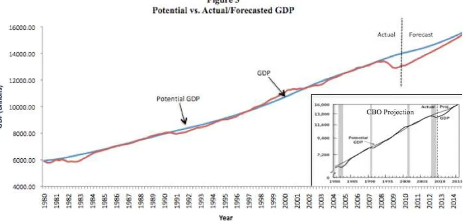
To provide further perspective on our findings, we compare the forecasts generated by our econometric models with the Congressional Budget Office’s (CBO) judgment-based projections of potential and projected GDP.10
Figure 3 maps the ARMA (2,1) models forecasted output path on top of the CBO’s potential GDP figures.
For comparison purposes, the CBO projection—which is also mapped on top of the potential GDP—is shown in the lower right panel of the figure. As we can see, our model predicts a similar recovery path to the projections made by the CBO
growth rates prior to the shock. This result seems unlikely given the structure of the experiment, and may
be attributable to the model’s complex roots. 10
The CBO’s economic projections are based on trends in the labor force, productivity, and saving. In
preparing its forecasts, the CBO examines and analyzes recent economic developments and relies on the
209
(although the CBO projections, which show projected GDP reaching potential GDP by 2015, seem slightly more optimistic) As we can see, our estimation techniques to measure the persistence of
the shock provide results highly
consistent with the CBO’s projected
recovery path. The findings, in
accordance with the CBO projections, suggest that the effects of the current shock may keep output levels below potential well into the upcoming decade.
Conclusions
Our findings of persistence
suggest that a current shock to the economy has longrun implications for future economic growth. According to Campbell and Mankiw, many traditional business cycle theorists, monetarists, and
neo-Keynesians maintain two
fundamental premises: (1) fluctuations in output are assumed to be driven primarily by shocks to aggregate demand, such as monetary or fiscal policy, and (2) shocks to aggregate demand are assumed to have only a temporary effect on output, and the economy returns to a natural growth rate in the long run (Campbell and Mankiw 1987).
However, if output shocks remain persistent into the foreseeable horizon, both of these premises cannot be strictly
maintained. Given the challenges
associated with distinguishing between a trend stationary process and a process that allows for permanent changes in
growth,11 we will discuss these premises and our results in light of several theoretical interpretations.
Nelson and Plosser argue against the first premise in favor of real business cycles, where fluctuations in output are attributable to changes and innovations
in aggregate supply, rather than
temporary demand shocks. They
abandon the notion that fluctuations are driven by aggregate demand— particularly monetary disturbances—
suggesting that technological
innovations are the source changes in economic growth patterns.
However, completely abandoning our first premise need not be necessary. For example, we can consider theories that attribute fluctuations to both supply and demand shocks. A Keynesian position may suggest that demand shocks affect supply, which, in turn, permanently effects on the economy. Similarly, it could be argued that demand shocks, in it of themselves, have permanent or near permanent effects.
Our second premise—shocks to aggregate demand are assumed to have only a temporary effect on output and the economy returns to a natural growth rate—can also be met be alternative theoretical interpretations. For example, models of multiple equilibria might explain a long-lasting effect of aggregate demand if shocks to aggregate demand
can move the economy between
11
For example, even if the output process is actually trend-stationary it may take quite a long time to get
210
equilibria (Diamond 1984). As well, the hysteresis theory suggests that supply or demand shocks may have permanent effects because they affect the natural rate of output, unemployment, inflation, etc. Thus, perhaps our findings of persistence suggest that there may be a “new” natural rate after an economic shock.
Although these theoretical
interpretations fall short of settling the
longstanding debate regarding the
existence of a unit root in the output process, they do provide context to our findings of persistence. While it remains challenging, if not impossible, to prove or disprove theories business cycles,
fluctuations, and output growth
behavior, our ARMA and Monte Carlo methods shift our efforts away from championing a single exclusive theory and towards realizing the impact and
persistence of economic shocks.
Works Cited
Bachman, Daniel, Peter Jaquette, Kurt Karl, and Pasquale Rocco. “The WEFA U.S. macro model with chain-weighted GDP.” Journal of Economic and Social
Measurement, 1998.
Blanchard, Oliver, and Mark Watson. “Are Business Cycles All Alike?” NBER
Working Paper Series. Working Paper
No. 1392, June 1984.
Campbell, John and Gregory Mankiw. “Are Output Fluctuations Transitory?”
The Quarterly Journal of Economics:
November 1987.
Christiano, Lawrence, and Martin
Eichenbaum. “Unit Roots in Real GNP:
Do We Know and Do We Care?” National
Bureau of Economic Research. October
1989.
Cochrane, John. “How Big is the Random Walk in GNP?” The Journal of Political
Economy, Vol. 96, No. 5. October 1988.
Diamond, Peter. A Search-Equilibrium, Approach to the Micro Foundations of
Macroeconomics. Cambridge,
Massachusetts: MIT Press, 1984.
Enders, Walter. Applied Econometric
Times Series, Second Addition. Wiley
Series in Probability and Statistics. 2004.
Evans, Martin. Where Are We Now?
Real-Time Estimates of the Macroeconomy.
International Journal of Central Banking, September 2005.
Jones, Charles. Sources of U.S. Economic
Growth in an World of Ideas. University
of California-Berkeley.
Lucas, Robert. Understanding Business
Cycles. Carnegie-Rochester Conference
on Public Policy. 1977.
Nelson, Charles, and Charles Plosser.
“Trends and Random Walks in
Macroeconomic Time Series: Some Evidence and Implications.” Journal of
211
Nelson, Charles, and Heejoon Kang. “Spurious Periodicity in Inappropriately Detrended Time Series: Some Evidence and Implications.” Journal of Monetary
Economics. 1982.
Papell, David, and Ruxandra Prodan. The
Uncertain Unit Root in U.S. Real GDP: Evidence with Restricted and Unrestricted
Structural Change. University of
Houston.
Romer, David. Advanced Macroeconomic.