Ordering Policy for Deteriorating Items with Time Dependent Demand

Vol. 7, No. 2, 2015, 177-184

ISSN: 2320 –3242 (P), 2320 –3250 (online) Published on 22 January 2015

www.researchmathsci.org

177

International Journal of

Ordering Policy for Deteriorating Items with Time

Dependent Demand

M. Maragatham1 and G. Gnanavel2 1

Department of mathematics, Periyar E.V.R. College, Trichy-23, India E-mail: [email protected]

Corresponding Author

2

Department of mathematics, SRG Engineering College, Namakkal-17, India E-mail: [email protected]

Received 30 October 2014; accepted 15 December 2014

Abstract. This paper deals with an inventory model to determine the optimal ordering quantity and optimal cycle time. It is assumed that the annual demand is a decreasing function of time and deteriorating units are replaced during the cycle time. Numerical examples are given to illustrate our results.

Keywords: Inventory model, deteriorating units, demand AMS Mathematics Subject Classification (2010): 90B05

1. Introduction

178

partial Backlogging. In this proposed study, an inventory model has been developed for deteriorating items. In this model deteriorating items are replaced under some conditions. The deteriorating items are constant and shortages are allowed in this model.

2. Notations and assumptions Notations

D(t) - The demand rate per unit time. θ _{- The deteriorating items per unit time.} H - The holding cost per unit.

C - The purchasing cost per unit time. Q - The ordering quantity.

A - The ordering cost per unit. T - The length of the cycle time.

C1 - The inventory shortage cost per unit time.

Tr - The replacement time for deteriorating items.

TC - The total present value of the cost over the cycle time.

Assumptions

1. The replenishment is uniform.

2. The shortage cost is a linear function of time D(t)=a(1-bt) If a>0 and 0<b>1.. 3. The holding cost is constant.

4. Shortages are allowed.

5.The deteriorating items are replaced when an inventory level reaches Q/2. 6. The purchasing cost of items used for replacement is C/2.

3. Mathematical formulation

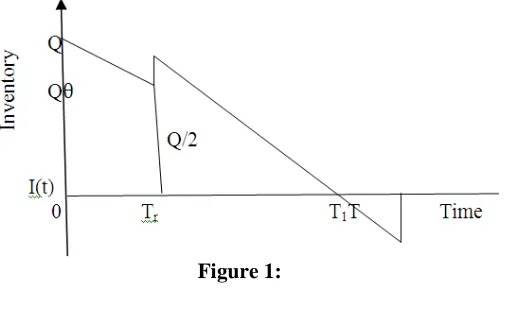
If the inventory model with above described assumption and notation is depicted in fig 1, we consider I(t) as total amount of inventory at the beginning of the each period. The variation of inventory level I(t) with respect to time t due to combined effect of demand and deterioration. But we have to replace the deteriorating items at Tr. Then inventory

level goes to zero at T1and shortages occur during time period(T1, T).The differential

equation in which on hand inventory I(t) satisfying in three different part of cycle time T are given by

179 ୢ୍ሺ୲ሻ

ୢ୲ + θIሺtሻ = −aሺ1 − btሻ 0 ≤ t ≤ T୰ (1) ୢ୍ሺ୲ሻ

ୢ୲ + θIሺtሻ = −aሺ1 − btሻT୰≤ t ≤ Tଵ (2) ୢ୍ሺ୲ሻ

ୢ୲ = −aሺ1 − btሻTଵ≤ t ≤ T (3)

dIሺtሻ

dt + θIሺtሻ = −aሺ1 − btሻ 0 ≤ t ≤ T୰ Iሺtሻe஘୲_{= −a නሺ1 − btሻe}஘୲_dt

Iሺtሻe஘୲_{= −a ቈ}ሺ1 − btሻe஘୲

θ +be

஘୲

θଶ ቉ + c

Iሺtሻe஘୲₌ିୟ

஘మሾθሺ1 − btሻ + bሿe஘୲+ c, where c is the constant of integration. The solution of equation (1), with boundary condition I(0)=Q, t=0

Q =−a_θଶሾθ + bሿ + c Q +_θa_ଶሾθ + bሿ = c Iሺtሻe஘୲₌−a

θଶሾθሺ1 − btሻ + bሿe஘୲+ Q +_θaଶሾθ + bሿ

Iሺtሻ =−a_θଶሾθሺ1 − btሻ + bሿ + Q + ቂ_θa_ଶሺθ + bሻቃ eି஘୲

Iሺtሻ = Q − θQt − at. (4) Thus the replacement time is obtained by putting the boundary condition t=Tr , I(Tr)=୕_ଶin

equation (1),

Q

2 = Q − θQT୰− aT୰ −Q_{2 = −θQT}୰− aT୰

_{ଶሺθ୕ାୟሻ}୕ = T_୰ (5)

During the period (Tr,T1) the inventory depletes due to the detoured or demand. Hence

the inventory level at any time during (Tr,T1) is described by differential equation. dIሺtሻ

dt + θIሺtሻ = −aሺ1 − btሻT୰≤ t ≤ Tଵ

Iሺtሻe஘୲_{= −a ቈ}ሺ1 − btሻe஘୲

θ +be

஘୲

θଶ ቉ + c

Iሺtሻ = −a ቈሺ1 − btሻ_θ +_θb_ଶ቉ + ceି஘୲

With the boundary condition when t=Tr , I(Tr)=୕_ଶ+ θQ, we have Qሺ1 + 2θሻ

2 = −a ቈሺ1 − bT୰

ሻ

θ +θbଶ቉ + ceି஘୘౨

ceି஘୘౨= a ቈሺ1 − bT୰ሻ

θ +θbଶ቉ +Qሺ1 + 2θሻ₂

c = e஘୘౨ቈa ቆሺ1 − bT୰ሻ

180

Iሺtሻ = −a ቈሺ1 − btሻ_θ +_θb_ଶ቉ + ቈa ቆሺ1 − bT_θ ୰ሻ+_θb_ଶቇ +Qሺ1 + 2θሻ₂ ቉ e஘ሺ୘౨ି୲ሻ

Iሺtሻ =୕ሺଵାଶ஘ሻ_ଶ + ቂa − abT୰+஘୕ሺଵାଶ஘ሻ_ଶ ቃ ሺT୰− tሻ (6) With the boundary condition t=T1 ,I(T1)=0

ܶଵ=

ொሺଵାଶఏሻ ଶ

ቂܽ − ܾܽܶ௥+ఏொሺଵାଶఏሻ_ଶ ቃ+ ܶ௥

ܶଵ=_{ሾଶ௔ሺଵି௕்}ொሺଵାଶఏሻ_{ೝሻାఏொሺଵାଶఏሻሿ}+ ܶ௥ (7) Thus the initial order quantity is obtained using the boundary conditions t=0 I(t)=Q

ܳ = −ܽ_{ߠ −}ܾܽ_ߠଶ+ܳሺ1 + 2ߠሻ₂ +ܽ_{ߠ −}ܾܽ_{ߠ ܶ}௥+ܾܽ_ߠଶ+ܳሺ1 + 2ߠሻߠܶ₂ ௥+ ܽܶ௥− ܾܽܶ௥ଶ+ܾܽ_{ߠ ܶ}௥

ܳ −ܳሺ1 + 2ߠሻ₂ −ܳሺ1 + 2ߠሻߠܶ₂ ௥= ܽܶ௥− ܾܽܶ௥ଶ

ܳ ൤1 −ሺ1 + 2ߠሻ₂ −ሺ1 + 2ߠሻߠܶ₂ ௥൨ = ܽܶ௥ሺ1 − ܾܶ௥ሻ

ܳ = ௔்ೝሺଵି௕்ೝሻ

ቂଵିሺభశమഇሻ_మ ିሺభశమഇሻഇ೅ೝ_మ ቃ (8) The state of inventory during (T1,T) can be represented by the differential equation.

݀ܫሺݐሻ

݀ݐ = −ܽሺ1 − ܾݐሻܶଵ≤ ݐ ≤ ܶ

ܫሺݐሻ = −ܽ නሺ1 − ܾݐሻ݀ݐ

ܫሺݐሻ = −ܽ ቆݐ −ܾݐ_{2 ቇ + ܿ}ଶ

With the boundary condition t=T1I(T1)=0

0 = −ܽ ቆܶଵ−ܾܶଵ ଶ

2 ቇ + ܿ ܿ = ܽ ቆܶଵ−ܾܶଵ

ଶ

2 ቇ

The solution of the equation is

ܫሺݐሻ = −ܽ ቆݐ −ܾݐ_{2 ቇ + ܽ ቆܶ}ଶ ଵ−ܾܶଵ ଶ

2 ቇ ܫሺݐሻ = ܽ ቈቆܶଵ−ܾܶଵ

ଶ

2 ቇ − ቆݐ −ܾݐ

ଶ

2 ቇ቉

ܫሺݐሻ = ܽ ቂሺܶଵ− ݐሻ −௕_ଶ൫ܶଵଶ− ݐଶ൯ቃ (9) The ordering cost is A. The total inventory holding cost during [0,T] is

ܪܥ = ℎ ቈන ܫሺݐሻ݀ݐ +்ೝ

଴ න ܫሺݐሻ݀ݐ

்భ

்ೝ

181

ܪܥ = ℎ ቈන ሺܳ − ߠܳݐ − ܽݐሻ݀ݐ்ೝ

଴

+ න ൤ܳሺ1 + 2ߠሻ₂ + ൤ܽ − ܾܽܶ௥+ߠܳሺ1 + 2ߠሻ₂ ൨ ሺܶ௥− ݐሻ൨ ݀ݐ ்భ

்ೝ

቉

ܪܥ = ℎ ቐቈܳܶ௥− ሺߠܳ − ܽሻܶ௥

ଶ

2 ቉ +ܳሺ1 + 2ߠሻ2 ሺܶଵ− ܶ௥ሻ

+ ൬ܽ − ܾܽܶ௥+ߠܳሺ1 + 2ߠሻ₂ ൰ ቌܶ௥ሺܶଵ− ܶ௥ሻ − ቆܶଵ ଶ

2 −ܶ௥

ଶ

2 ቇቍቑ ܪܥ = ℎ ቄቂܳܶ௥− ሺߠܳ − ܽሻ்ೝ

మ

ଶ ቃ +ொሺଵାଶఏሻଶ ሺܶଵ− ܶ௥ሻ + ቀܽ − ܾܽܶ௥+ఏொሺଵାଶఏሻଶ ቁ ቀܶଵܶ௥− ்భమ

ଶ −்ೝ మ

ଶቁቅ (10) The shortage cost during [ T1,T]

ܵܥ = ܥଵቈන ܫሺݐሻ݀ݐ

்

்భ

቉

ܵܥ = ܥଵܽ ቈන ൤ሺܶଵ− ݐሻ −ܾ_{2 ൫ܶ}ଵଶ− ݐଶ൯൨ ݀ݐ ்

்భ

቉

ܵܥ = ܥଵܽ ቎ቌܶଵሺܶ − ܶଵሻ − ቆܶ ଶ_{− ܶ}

ଵଶ

2 ቇቍ −ܾ2 ቌܶଵଶሺܶ − ܶଵሻ − ቆܶ

ଷ_{− ܶ} ଵଷ

3 ቇቍ቏

ܵܥ = ܥଵܽ ቈܶଵܶ −ܶଵ ଶ

2 −ܶ

ଶ

2 −ܾ2 ቆܶଵଶܶ −2ܶ

ଷ

3 −ܶଵ

ଷ

3 ቇ቉ ܵܥ = ܥଵܽ ൤ܶଵܶ −ሺ்భ

మ_ା்మ_ሻ

ଶ −

௕

ଶቀܶଵଶܶ −

ሺଶ்య_ି்భయ_ሻ

ଷ ቁ൨ (11) The purchasing cost during [0, T1]

ܲܥ = ܥܳ + ߠܳܥ₂

ܲܥ =ொ஼_ଶ ሺ2 + ߠሻ (12) The total cost per unit time TC (T) is

ܶܥሺܶሻ =_{ܶ ሾܱܥ + ܵܥ + ܲܥ + ܪܥሿ}1

Now TC (T) will be minimum whenడ்஼ሺ்ሻ_డ் = 0 andడమ_డ்்஼ሺ்ሻ_మ > 0 , ܶhe optimum values of T for the minimum average total cost TC(T) is the solution of equation

182

߲ܶܥሺܶሻ

߲ܶ = −ܶܣଶ

−_ܶℎ_ଶቊቈܳܶ௥− ሺߠܳ − ܽሻܶ௥ ଶ

2 ቉ +ܳሺ1 + 2ߠሻ2 ሺܶଵ− ܶ௥ሻ + ൬ܽ − ܾܽܶ௥+ߠܳሺ1 + 2ߠሻ₂ ൰ ቆܶଵܶ௥−ܶଵ

ଶ

2 −ܶ௥

ଶ

2 ቇቋ −ܳܥܶଶሺ2 + ߠሻ₂

+ ܥଵܽ ቌܶଵ ଶ

2ܶଶ−1_{2 −}ܾ_{2 ቆ}2ܶଵ ଷ

3 −2ܶ3 ቇቍ = 0

−_ܶܣ_ଶ−_ܶℎ_ଶቊቈܳܶ௥− ሺߠܳ − ܽሻܶ௥ ଶ

2 ቉ +ܳሺ1 + 2ߠሻ2 ሺܶଵ− ܶ௥ሻ + ൬ܽ − ܾܽܶ௥+ߠܳሺ1 + 2ߠሻ₂ ൰ ቆܶଵܶ௥−ܶଵ

ଶ

2 −ܶ௥

ଶ

2 ቇቋ −ܳܥܶଶሺ2 + ߠሻ₂

+ܥ_ܶଵ_ଶܽቆܶ_{2 −}ଵଶ 2ܶ_{3 ቇ + ܥ}ଵଷ ଵܽ ൬ܾܶ_{3 −}1_{2൰ = 0}

ܶଶ_ܥ

ଵܽ ൬ܾܶ_{3 −}1_2൰

= ܣ

+ ℎ ቊቈܳܶ௥− ሺߠܳ − ܽሻܶ௥ ଶ

2 ቉ +ܳሺ1 + 2ߠሻ2 ሺܶଵ− ܶ௥ሻ + ൬ܽ − ܾܽܶ௥+ߠܳሺ1 + 2ߠሻ₂ ൰ ቆܶଵܶ௥−ܶଵ

ଶ

2 −ܶ௥

ଶ

2 ቇቋ + ܳܥሺ2 + ߠሻ2 − ܥଵܽ ቆܶଵ

ଶ

2 −2ܶଵ

ଷ

3 ቇ

ሺ2ܾܶଷ_{− 3ܶ}ଶ_{ሻ =} 6

ܥଵܽ ቊܣ

+ ℎ ቊቈܳܶ௥− ሺߠܳ − ܽሻܶ௥ ଶ

2 ቉ +ܳሺ1 + 2θሻ2 ሺTଵ− T୰ሻ + ቆa − abT୰+θQሺ1 + 2θሻ₂ ቇ ቆTଵT୰−Tଵ

ଶ

2 −T୰

ଶ

2 ቇቋ + QCሺ2 +

θሻ

2 − Cଵa ቆTଵ

ଶ

2 −2Tଵ

ଷ

3 ቇቋ

Provided that it satisfies the following conditions

∂ଶ_TCሺTሻ

∂Tଶ =2A_Tଷ+2h_TଷቊቈQT୰+ θQሺa − 1ሻT୰ ଶ

2 ቉ +Qሺ1 + 2θሻ2 ሺTଵ− T୰ሻ + ቆaሺ1 − bT୰ሻ +θQሺ1 + 2θሻ₂ ቇ ቆሺTଵ−T୰ሻ

ଶ

2 ቇቋ +2QCTଷ ሺ2 + θሻ₂

183 பమ_{୘େሺ୘ሻ}

ப୘మ > 0, [Tଵ> T୰, 3 > 2ܾTଵ, a > 1,(Therefore its terms are positive)]

3.1. Numerical examples

Example 3.1.1. Let a=100 units/year b=0.2, A=100 per order, C=8 per unit, C1=100 per

unit, h=60 unit/annum, θ_{=0.2 by the help of mathematical calculations, we obtain the} optimum solutions are Q*= 150 and T*= 1.5 putting Q* and T* we get the optimum average cost TC (T)*=3297.

Example 3.1.2. Let a=400 units/year=0.2, A=100 per order, C=8 per unit, C1=100 per

unit, h=60 unit/annum, θ_{=0.2 by the help of mathematical calculations, we obtain the} optimum solutions are Q*=603 and T*=1.9 putting Q* and T* we get the optimum average cost TC (T)*=10226.

5. Conclusion

In this paper, an inventory model is developed in which annual demand is decreasing function of time and deteriorating items are replaced during the cycle time. This model is solved analytically by minimizing the total cost finally; the proposed model is verified by the numerical example.

REFERENCES

1. H.Bahari Kashani, Replenishment schedule for deteriorating items with time proportional demand, Journal of Operation Research Society, 40 (1989) 95-81. 2. H.J.Chang and C.Y.Dye, An Inventory model for deteriorating items with linear

demand under condition of permissible delay in payments, Production Planning and Control, 12 (2001) 274-282.

3. K.J.Chung and Y.F.Hway, The optimal cycle time for EOQ inventory model under permissible delay in payments, International Journal of Production Economics, 84 (2003) 307-318.

4. U.Deva and L.K.Patel, (T, Si) Policy inventory model for deteriorating item with time proportional demand, J. Opl. Res. Soc., 32 (1981) 137-142.

5. P.M.Ghare and G.F.Schrader, A model for an exponentially decaying inventory, Journal of Industrial Engineering, 14 (1963) 238-243.

6. S.K.Goyal and B.C.Giri, Recent trends in modeling of deteriorating inventory, Euoropean J. Operational Research, 134 (2001) 1-16.

7. F.W.Harish, Operations and cost, A.W.Company, Chicago,1951.

8. M.Maragatham and P.K.Lakshmidevi, An inventory model for non-instantaneous deterioratingitems under conditions of permissible delay in paymentsfor n-cycles, Intern. J. Fuzzy Mathematical Archive, 2(2013) 49-57. 9. M.Kumar, A.Chauhan and R.Kumar, A deterministic inventory model for

deteriorating items with price dependent demand and time varying holding cost under trade credit, International Journals of Soft Computing and Engineering, 2 (2012).

184

11. S.Singh, An Economic order quantity model for item having linear demand under inflation and permissible delay, International Journals of Computer Applications, 33 (9) (2011) 520-527.

12. Y.K.Shah and M.C.Jaiswal, A lot size model for exponentially deteriorating inventory with finite production rate, European J. Operational Research, 29 (1976) 70-72.

13. T.Singh and H.Pattnayk, An EOQ model for deteriorating items with linear demand, variable deterioration and partial backlogging, Journals of Service Science and Management, 6 (2) (2013) 186-190.

14. R.P.Tripathy and A.K.Uniyal., A quantiy dependent EOQ model with cash flow under permissible delay in payments, IJSTM, 2 (2011) 20-26.