Vol.6 (2016) No. 4
ISSN: 2088-5334
Splines in Compressed Sensing
S.Abhishek
#, S.Veni
#, K.A Narayanankutty
# #Department of Electronics &Communication Engineering, Amrita School of Engineering, Coimbatore Amrita VishwaVidyapeetham, Amrita University, 641112, India
E-mail: [email protected], [email protected], [email protected]
Abstract— It is well understood that in any data acquisition system reduction in the amount of data reduces the time and energy, but the major trade-off here is the quality of outcome normally, lesser the amount of data sensed, lower the quality. Compressed Sensing (CS) allows a solution, for sampling below the Nyquist rate. The challenging problem of increasing the reconstruction quality with less number of samples from an unprocessed data set is addressed here by the use of representative coordinate selected from different orders of splines. We have made a detailed comparison with 10 orthogonal and 6 biorthogonal wavelets with two sets of data from MIT Arrhythmia database and our results prove that the Spline coordinates work better than the wavelets. The generation of two new types of splines such as exponential and double exponential are also briefed here .We believe that this is one of the very first attempts made in Compressed Sensing based ECG reconstruction problems using raw data.
Keywords— Compressed Sensing; Splines; 2E Splines; PRD; SNR
I. INTRODUCTION
In normal conditions reasonable reconstruction quality can be assured by maintaining the Nyquist rate[1], but sampling below Nyquist rate is always an attractive option especially in situations where collection of samples are too costly or physically not possible to collects the samples at the rate Nyquist demands [2].To deal with these situations people usually does compression which finds the abridged representation of the data which is capable of doing an acceptable reconstruction at the receiver side. Transform coding [3], one of the most used techniques in compression aims finds an alternative set of basis where the signal has a sparse representation. For a signal of length ‘n’, if it has only ‘k’ non-zero coefficients, in a domain of interest then is said to have a sparsity of ‘k’ in that domain. Such a signal can be recovered accurately with the knowledge of only ‘k’ (or less than ‘k’) non-zero coefficients. This is often called as sparse approximation which is the basis idea behind transform coding. Inspiring from the idea of sparse approximation a new concept called Compressed Sensing (CS) was formulated which ensures reasonable approximation even with sensing fewer measurements lesser than Nyquist rate. The basic idea behind CS is relatively simple, if the signal is sparse in a basis then why we do sense all the information? Rather than sensing all the information and the throwing the unwanted ones why do we find methods to sense the data in the compressed form itself. Even though this idea came to limelight after the publication of the papers by Candes,
Fig.1 B-spline, Linear spline (triangle), Quadratic and Cubic spline.
There are lots of papers published in the field of CS based ECG reconstruction most of them considers CS as a technique for compression rather than a sensing paradigm [12-17]. Recently in May-2015 Abo-Zahhad, et.al published their work [18] which is showing some promising results, In that they have estimated the QRS complex from the available data and subtracted it from the original and CS techniques are applied on the error signal. The major drawback here is that prior information of the data has to known before, and thresholding has also been employed to increase sparsity. Preprocessing techniques like smoothening, removal of dc offset and thresholding to improve the quality of data are actually contradictory to the original CS based approach. In ideal CS based reconstruction scenario, we sense only a few random coefficients and the algorithm is expected to reconstruct the original signal without sensing the whole data points. As it sounds magical the convex optimization algorithm used in CS is often known as l1 magic [19]. So in our work, none of the preprocessing methods are applied on the data and have included a low-frequency base to capture low-low-frequency information. We had selected spline coordinates instead of wavelet basis and made a detailed comparison between the two. Spline coordinates are compared against the wavelet basis and it was found out that the splines work better than wavelets. The exponential spline is kind of splines which uses causal exponentials instead of polynomials were introduced by Unser. M et.al in 2005 [20] and double sided exponentials spline family [2E spline] was introduced by us through our earlier work [21]. 2E spline uses two-sided exponentials fragments for generating higher orders.
The remaining of the paper is arranged as follows: Section II gives a brief introduction of CS theory, Section III deals with splines, where a brief description of polynomial, exponential, and double exponential spline families are given in subsections. In Section IV, the details about the construction of sparsifying matrix from the spline coordinates are discussed. Results are analyzed in Section V and in subsection the effect of the addition of dc base in the sparsifying domain are detailed; we conclude this paper in section VI
Fig.2 Causal Exponent with an exponential factor of 1. This can be used for the generation of higher order exponential splines.
II. COMPRESSED SENSING (CS)
As mentioned, CS theory states that if the signal has a sparse representation in a certain domain then it can be recovered using a small number of coefficients lesser than that of Nyquist rate by solving basis pursuit algorithms or using greedy based algorithms. For example consider ‘x’ as the input vector of size N x 1, and if it has a sparse representation in a domain say ‘β’ with coefficients as ‘ , mathematically the problem of finding from the measurements ‘y’ can be formulated as
(1) s.t y= .
Where ‘y’ represents the random samples collected by projecting ‘x’ on a sensing matrix Φ, and is called as the reconstruction matrix which is the product of Φ and β i.e.
β, dimensions of Φ is ‘M x N’, where ‘M’ represents the number of projected samples, and ‘β’ is of size N x N; where N is the signal length. The reconstruction matrix (‘ will be of size ‘M x N’. The transform matrix β can be discrete cosine basis or wavelets basis or any other basis in which the signal is supposed to have a sparse representation. In this present work, we have compared this matrix (β) using basis selected from different orders of spline with orthogonal and biorthogonal wavelets. The problem of finding the sparsest solution using l0 norm is NP-hard, computationally not possible to solve in real time [ 22].But CS theory states that this problem can be relaxed in the form
Min (2)
s.t y= .
CS seems to be a better option it is still underutilized in ECG-based applications, this may be because of unavailability of proper hardware in capturing the real-time data, which is always a challenging problem. Some research in recent years [29-30] based on random demodulation changed the scenario and CS is more attractive than before. Random demodulators can be used to collect the random samples instead of sensing the whole signal. Recently Bortolotti et .al proposed an ECG monitor based on CS architecture which saves up to 70% of power compared to other monitors [31].
III.POLYNOMIAL AND EXPONENTIAL SPLINES
Michael Unser made a series of publications [32-37] in spline fitting theory which showcases the advantageous of splines in signal and image processing. A discrete signal can be well approximated using splines, and polynomial splines can be constructed from B-spline basis functions. If the spline knots are placed at equally spaced integers, its parameters can be found by simple digital filtering rather than complex matrix manipulations. The spline is one of the most flexible functions, i.e. by increasing the degree of the spline (n) we can progressively switch from the constant (n=0) and piecewise linear representations (n=1) to the other extremes n=∞, i.e. up to band limited models. Three different types of splines are detailed such as polynomial, exponential, and double exponential splines.
Fig.3. 0th, 1st, 2nd, and 3rd order Exponential splines.
A. Polynomial splines
A polynomial spline (spline) is a numeric function that is piecewise defined by polynomial functions. They possess a high degree of smoothness at the points where these polynomial segments are connected. These points are called as knots. The individual segments are polynomials and this characteristic of splines make them a better contender in approximation problems,
The Polynomial B-spline of order zero can be obtained from rectangular function
0(y) =
Polynomial splines are obtained by connecting polynomial of degree one or by connecting straight lines.
In quadratic spline, the individual segments will be connected by polynomial of degree 2, for example
2(y) =
Cubic spline, most commonly used splines in interpolation problems can be represented as
B3(y)= (5)
The linear, quadratic, cubic splines and the basis spline (B-Spline) are shown in Figure.1
Higher order splines can be obtained by the repetitive convolution of the lower order ones [20].
B n(y) = B0 (y)* B 1(x)* B 2(y)*…..* Bn-1(y) (6)
B. Exponential Splines
Exponential Splines were introduced in order to reduce the gap between the spline fitting and continuous system theory. Here in exponential splines instead of polynomials, cardinal causal exponentials are connected in smooth fashion. Instead of rectangular function here an exponent in unit interval is used as basis function (B0y) for generating higher
order splines. Similar to polynomial splines higher order splines are obtained by the convolution of lower order splines. B- spline used for exponential splines with a factor of one is shown in Figure [2] and Figure[3] shows zero, first, second and third order causal exponential splines
C. Double Sided exponential Splines
We tried exponential splines in our experiment and found that the splines are not symmetric in nature so we developed a new family of symmetric splines called double sided exponential splines. The basis function used for generating – this type of spline is of the form (where ‘a’ indicates the scaling parameter and b, the index of the central (maximum) point)).Higher order splines can be obtained from the convolution of the basis function. This can be called as 2E splines.
The first, second, third order double-sided exponential splines along are shown in Figure [4]. From the figure it can be observed that the spline obtained from double sided exponents shows symmetric characteristics as compared to asymmetric nature of splines obtained from causal exponents.
IV.ALGORITHM FOR CONSTRUCTING SPARSIFYING MATRIX FROM SPLINES.
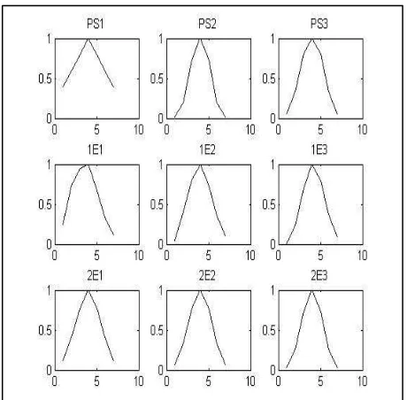
Sparsifying matrices are constructed by taking the representative coordinates from both the first, second, third order exponential, double exponential and polynomial splines. The points are selected in such a way that they are at equal distance from the center of the spline. The polynomial and double exponential spline coordinates are symmetric in nature because of the symmetric nature of their splines, where exponential spline coordinates are asymmetric in nature. The coordinates selected are shown in Table.1.We dictate asymmetrical exponential splines as one-sided exponential splines or 1E splines and symmetrical exponential splines as double sided splines or 2E splines. We introduced a low frequency/dc base, for capturing the low-frequency information so, if the data (to be reconstructed) is having a DC content that also will be reconstructed. This seems to be very much important as in practical cases as it will not be possible to take samples without having a DC content at least in sensor outs. The reasoning behind this is that bio measurements like ECG employ the same number of electrodes expecting the half cell potential [38] to cancel out. But in practical cases difference in electrode material or skin contact resistance causes a DC offset voltage which makes deviations or baseline drift in the readings. In ideal CS we are expected to collect only a few random samples (not the complete signal) and the algorithm is expected to construct the original data from the limited data sensed. So if we are collecting few samples from a preprocessed data for experimental purpose and analyzing the result based on that, we can only presume that the algorithm will work fine if the data (to be reconstructed) contains dc artifacts. Moreover, rather than reconstructing the original data in the domain where the data is sensed, the CS algorithms recover coefficients of the signal in the domain where it is having a sparse representation (provided if the data does not have a sparse representation in the sensing domain.). There is no guarantee that the random samples sensed with or without noise will have the same sparse presentation in the alternate domain. Moreover Józef K. Cywiński et.al [39] points that very low frequency and DC components of ECG signal carry information about the heart muscle conditions. Different splines tried in our problem are as follows:
PS1 - First order polynomial spline, PS2 - Second order polynomial spline, PS3-Third order Polynomial Spline (cubic Spline), 1E1- First order one-sided exponential spline, 1E2- Second order one-sided exponential spline,1E3- Third order one-sided exponential spline, 2E1- First order double-sided exponential spline, 2E2- Second order double-double-sided exponential spline, 2E3- Third order double-sided exponential spline.
V. RESULTS AND DISCUSSIONS
The algorithm is analyzed on the basis the important parameters such as Percentage Root mean square Difference (PRD) and Signal to Noise Ratio (SNR) and Compression Ratio (CR) which are used to quantify the error between the original and reconstructed signal. The formulation of PRD is given in equation (5)
Where be the original signal, be the reconstructed signal and N be its length. CR is defined as the ratio between the numbers of bits used for representing the uncompressed signal to the bites in compressed signal
Where orig and comp represent the number of bits required for the original and compressed signals respectively. SNR can be found from PRD using relation
SNR= - 20log10 (0.01 × PRD) (7)
TABLEI
DIFFERENT SPLINES AND THE COORDINATES SELECTED.
Ratios for the MIT data 101m, Table.3 indicate the same for 101m. Table 4 and Table 5 indicate corresponding SNR values for 101m and 104m respectively. A low PRD and higher SNR are indicating good reconstruction. From Tables 2, 3, 4, 5 it is evident that Splines coordinates perform better than wavelets.
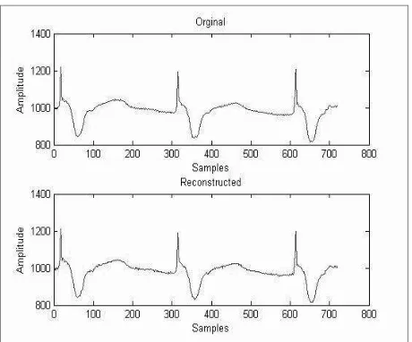
A sample of reconstructed data for the first 720 samples from the data set 101 using first order spline coordinates are shown in Fig.6. and Figure .7 indicate the same for 104
VI.EFFECT OF LOW-FREQUENCY BASE IN RECONSTRUCTION MATRIX
Even though the introduction of a low-frequency base in the transform matrix successively capture low-frequency information from the projected samples it has some adverse effect on the reconstruction matrix, upon performing decomposition using SVD (Singular Value Decomposition), it was found that the introduction of dc base shoots up the first singular value and makes the condition number worse. This is because the addition of a dc base in transform domain replaces a column in reconstruction matrix by the sum of column elements of the sensing matrix. The increase in singular value normally deteriorates the matrix. But here increase in singular value does not have any effect on reconstruction quality; this is proved by reconstructing the signal using unmodified matrix singular values. Our experiments show that increase in first singular value doesn’t have an effect and the reconstruction quality is still preserved even though the first singular value is lowered down. Singular value of the reconstruction matrix with and without a dc base along the sparsifying basis is shown below. Figure 8.a shows the singular values (SV) of the reconstruction with adding a dc base along the sparsifying bases and figure 8.b shows the singular values of the reconstruction matrix when a dc base is added. In the first case the maximum SV is 140 and in the second case, it is 698
Fig.5 Different representative coordinates selected from polynomial and exponential splines. PS1 - First order polynomial spline,PS2 - Second order polynomial spline,PS3-Third order Polynomial Spline (cubic Spline),1E1- First order one-sided exponential spline,1E2- Second order one-sided exponential spline,1E3- Third order one-sided exponential spline,2E1- First order double-sided exponential spline,2E2- Second order double-sided exponential spline,2E3- Third order double-sided exponential spline.
Fig.6 The original data (top) and the reconstructed data using first order spline coordinates (1E1) for data set 101m by sensing only 30% of the samples.
Spline Type Representative coordinates selected
First order polynomial Spline(PS1) 0.4, 0.6, 0.8, 1, 0.8, 0.6, 0.4
Second order Polynomial spline(PS2) 0.0133,0.2, 0.733,1,0.733,0 .2,0.0133
Fig.7 The original data (top) and the reconstructed data using first order spline coordinates (1E1) for data set 107m
Fig. 8a.Singular Value of the reconstruction matrix without a dc base
Fig. 8b.Singular value of the reconstruction matrix with dc base
TABLEII
PRD OBTAINED FOR THE DATA 101.MFROM MIT DATA BASE FOR DIFFERENT WAVELETS AND SPLINE COORDINATES
Compression
Ratio(CR) 10 20 30 40 50 60
Wavelet Filter
db1 3.54 2.35 1.75 1.30 1.02 0.80
db2 3.85 2.54 1.92 1.55 1.25 0.95
db3 4.46 2.93 2.20 1.68 1.49 1.12
db4 3.98 2.95 2.15 1.75 1.35 0.95
db5 3.85 2.80 2.35 1.91 1.21 1.02
db6 3.65 2.25 1.95 1.43 1.20 0.92
db7 3.71 2.37 1.65 1.50 1.32 1.02
db8 4.22 2.95 2.48 1.55 1.54 0.95
db9 3.65 3.25 2.35 1.64 1.24 0.83
db10 3.02 2.13 1.52 0.83 0.65 0.50
bior1.1 3.23 2.65 1.88 1.42 1.12 0.85
bior1.3 3.62 2.56 2.32 1.66 1.23 0.85
bior1.5 3.52 2.46 1.92 1.52 1.13 0.72
bior2.2 3.71 2.56 1.84 1.75 1.44 0.84
bior2.4 3.62 2.86 2.15 1.36 1.02 0.71
bior2.6 3.40 2.75 2.58 1.82 1.18 0.91
bior2.8 3.32 2.45 2.25 1.65 1.21 0.95
bior3.9 3.59 2.35 2.45 1.72 1.35 1.02
bior4.4 3.25 2.23 1.65 1.15 0.75 0.52
bior5.5 4.01 3.64 2.55 1.91 1.38 1.12
bior6.8 3.85 2.82 2.42 1.65 1.25 0.81
PS1 2.85 2.34 1.73 1.25 0.85 0.43
PS2 2.75 2.45 1.94 1.32 0.76 0.34
PS3 2.88 2.14 1.76 1.28 0.83 0.43
1E1 1.91 1.42 0.95 0.49 0.35 0.18
1E2 1.74 1.35 0.81 0.55 0.24 0.12
1E3 1.95 1.35 0.95 0.61 0.27 0.28
2E1 1.85 1.22 0.72 0.55 0.32 0.15
2E2 1.66 1.15 0.92 0.49 0.21 0.15
2E3 1.81 1.22 0.82 0.41 0.19 0.09
PRD-101.m
TABLEIII
PRD OBTAINED FOR THE DATASET 104.MFROM MIT DATA BASE FOR DIFFERENT WAVELETS AND SPLINE COORDINATES
Compression
Ratio(CR) 10 20 30 40 50 60
Wavelet Filter
db1 3.65 2.24 1.61 1.25 1.14 0.74
db2 3.50 2.35 2.12 1.66 1.15 0.81
db3 4.24 2.72 1.93 1.52 1.03 0.80
db4 3.85 2.75 2.35 1.82 1.24 0.93
db5 3.62 2.50 2.16 1.74 1.46 1.13
db6 3.95 2.45 2.04 1.32 1.10 0.85
db7 3.46 2.65 1.93 1.42 1.43 1.15
db8 3.85 2.75 2.35 1.31 1.15 0.80
db9 3.32 2.65 2.11 1.55 1.22 0.85
db10 3.02 1.92 1.60 0.91 0.55 0.35
bior1.1 3.32 2.75 1.75 1.35 1.02 0.75
PRD-104.m
bior1.1 3.32 2.75 1.75 1.35 1.02 0.75
bior1.3 3.55 2.72 2.16 1.52 1.12 0.80
bior1.5 3.72 2.65 2.01 1.38 1.04 0.82
bior2.2 3.88 2.45 1.72 1.42 1.25 0.65
bior2.4 3.55 2.70 2.28 1.74 1.14 0.72
bior2.6 3.45 2.57 2.15 1.63 1.36 0.95
bior2.8 3.39 2.45 2.03 1.52 1.30 0.81
bior3.9 3.45 2.65 2.45 1.68 1.27 0.98
bior4.4 3.12 2.30 1.60 1.04 0.84 0.43
bior5.5 3.83 3.34 2.44 1.85 1.43 1.24
bior6.8 3.75 3.02 2.35 1.55 1.18 0.75
PS1 2.63 2.15 1.63 1.32 0.75 0.51
PS2 2.52 2.05 1.83 1.25 0.87 0.56
PS3 2.46 2.26 1.93 1.39 0.73 0.61
1E1 1.99 1.52 0.85 0.63 0.42 0.28
1E2 1.75 1.26 0.62 0.42 0.32 0.20
1E3 1.81 1.45 0.95 0.72 0.29 0.13
2E1 1.71 1.50 0.85 0.61 0.32 0.20
2E2 1.62 1.26 0.72 0.51 0.31 0.21
2E3 1.85 1.55 0.95 0.42 0.25 0.15
TABLEIV
SNR CALCULATED FOR THE DATASET 101.MFROM MIT DATA BASE FOR DIFFERENT WAVELETS AND SPLINE COORDINATES
Compression
Ratio(CR) 10 20 30 40 50 60
Wavelet Filter
db1 29.03 32.59 35.14 37.71 39.79 41.94
db2 28.30 31.92 34.32 36.22 38.09 40.49
db3 27.02 30.65 33.16 35.52 36.56 38.99
db4 28.01 30.61 33.36 35.15 37.41 40.46
db5 28.30 31.07 32.59 34.36 38.33 39.79
db6 28.77 32.96 34.22 36.92 38.45 40.74
db7 28.61 32.52 35.67 36.49 37.56 39.79
db8 27.50 30.61 32.12 36.21 36.22 40.46
db9 28.76 29.77 32.58 35.73 38.12 41.58
db10 30.40 33.42 36.35 41.57 43.79 46.10
bior1.1 29.81 31.54 34.54 36.93 38.98 41.44
bior1.3 28.83 31.82 32.71 35.58 38.17 41.46
bior1.5 29.08 32.20 34.35 36.39 38.97 42.90
bior2.2 28.60 31.82 34.73 35.14 36.86 41.50
bior2.4 28.83 30.88 33.35 37.35 39.79 42.93
bior2.6 29.38 31.22 31.77 34.82 38.56 40.80
bior2.8 29.59 32.23 32.96 35.65 38.32 40.48
bior3.9 28.90 32.56 32.23 35.31 37.42 39.79
bior4.4 29.77 33.02 35.66 38.80 42.53 45.74
bior5.5 27.93 28.77 31.87 34.37 37.23 39.05
bior6.8 28.29 31.01 32.34 35.63 38.09 41.79
PS1 30.91 32.63 35.22 38.09 41.44 47.31
PS2 31.22 32.22 34.24 37.62 42.34 49.39
PS3 30.83 33.37 35.07 37.86 41.57 47.43
1E1 34.36 36.93 40.48 46.24 49.00 54.98
1E2 35.21 37.40 41.78 45.21 52.56 58.79
1E3 34.22 37.40 40.43 44.26 51.32 51.21
2E1 34.68 38.30 42.90 45.25 50.00 56.59
2E2 35.62 38.75 40.76 46.12 53.37 56.54
2E3 34.83 38.25 41.77 47.65 54.24 60.49
SNR
TABLEV
SNR CALCULATED FOR DATASET 104.MFROM MIT DATA BASE FOR DIFFERENT WAVELETS AND SPLINE COORDINATES
Compression
Ratio(CR) 10 20 30 40 50 60
Wavelet Filter
db1 28.76 32.98 35.85 38.10 38.85 42.67
db2 29.11 32.59 33.46 35.62 38.80 41.81
db3 27.46 31.32 34.31 36.39 39.79 41.95
db4 28.30 31.22 32.60 34.79 38.17 40.59
db5 28.84 32.03 33.33 35.17 36.72 38.97
db6 28.08 32.23 33.82 37.58 39.19 41.44
db7 29.23 31.55 34.31 36.98 36.87 38.80
db8 28.29 31.22 32.59 37.64 38.75 41.95
db9 29.59 31.55 33.50 36.20 38.30 41.42
db10 30.41 34.35 35.91 40.78 45.20 49.23
bior1.1 29.57 31.23 35.14 37.42 39.79 42.55
bior1.3 29.01 31.32 33.31 36.34 38.99 41.99
bior1.5 28.60 31.55 33.93 37.17 39.70 41.68
bior2.2 28.23 32.23 35.31 36.94 38.09 43.76
bior2.4 29.00 31.39 32.84 35.18 38.83 42.80
bior2.6 29.25 31.79 33.35 35.78 37.35 40.47
bior2.8 29.40 32.23 33.83 36.34 37.73 41.78
bior3.9 29.25 31.54 32.23 35.52 37.93 40.13
bior4.4 30.10 32.76 35.93 39.70 41.57 47.40
bior5.5 28.33 29.52 32.27 34.68 36.88 38.16
bior6.8 28.51 30.39 32.59 36.20 38.57 42.55
PS1 31.59 33.37 35.73 37.57 42.55 45.81
PS2 31.99 33.78 34.73 38.07 41.26 44.96
PS3 32.18 32.90 34.31 37.14 42.68 44.23
1E1 34.04 36.39 41.46 44.06 47.54 51.00
1E2 35.16 37.97 44.20 47.60 50.03 54.20
1E3 34.83 36.80 40.48 42.91 50.66 57.96
2E1 35.32 36.50 41.45 44.23 50.03 54.20
2E2 35.80 37.97 42.90 45.81 50.12 53.45
2E3 34.68 36.22 40.48 47.63 52.19 56.72 SNR
VII. CONCLUSIONS
REFERENCES
[1] H. Nyquist. Certain topics in telegraph transmission theory. Trans. AIEE, 47:617–644, 1928.
[2] R. Walden. Analog-to-digital converter survey and analysis. IEEE J. Selected Areas Comm., 17(4):539–550, 1999.
[3] Pratt, W.; Kane, J.; Andrews, Harry C., "Hadamard transform image coding," in Proceedings of the IEEE , vol.57, no.1, pp.58-68, Jan. 1969.
[4] E. J. Candès, J. Romberg, and T. Tao, Robust uncertainty principles: Exact signal reconstruction from highly incomplete frequency information. IEEE Trans. Inform. Theory, 52(2) pp. 489–509, February 2006.
[5] E. J. Candès, and J. Romberg, Quantitative robust uncertainty principles and optimally sparse decompositions. Foundations of Comput. Math., 6(2), pp. 227–254, April 2006.
[6] E. J. Candès, and T. Tao, Near optimal signal recovery from random projections: Universal encoding strategies? IEEE Trans. Inform. Theory, 52(12), pp. 5406–5425, December 2006.
[7] B. Kashin, The widths of certain finite dimensional sets and classes of smooth functions, Izvestia 41(1977), 334–351.
[8] A. M. Pinkus, N-widths in Approximation Theory.Ergeb.Math.Grenzgeb. (3) 7, Springer-Verlag, Berlin 1985. [9] [Unattributed]: Prony Analysis: [ http://www.engr.uconn.edu/
~sas03013/docs/PronyAnalysis.pdf.]
[10] Fensli, R.; Gunnarson, E.; Hejlesen, O., "A wireless ECG system for continuous event recording and communication to a clinical alarm station," in Engineering in Medicine and Biology Society, 2004. IEMBS '04. 26th Annual International Conference of the IEEE , vol.1, no., pp.2208-2211, 1-5 Sept. 2004
[11] Ravelomanantsoa, A.; Rabah, H.; Rouane, A., "Simple and Efficient Compressed Sensing Encoder for Wireless Body Area Network," in Instrumentation and Measurement, IEEE Transactions on , vol.63, no.12, pp.2973-2982, Dec. 2014.
[12] Mishra, A.; Thakkar, F.; Modi, C.; Kher, R., "ECG signal compression using Compressive Sensing and wavelet transform," in Engineering in Medicine and Biology Society (EMBC), 2012 Annual International Conference of the IEEE , vol., no., pp.3404-3407, Aug. 28 2012-Sept. 2012
[13] Chen, Fred, Anantha P. Chandrakasan, and Vladimir M. Stojanovic. "Design and analysis of a hardware-efficient compressed sensing architecture for data compression in wireless sensors." Solid-State Circuits, IEEE Journal of 47, no. 3 (2012): 744-756.
[14] Polania, L.F.; Carrillo, R.E.; Blanco-Velasco, M.; Barner, K.E., "Compressed sensing based method for ECG compression," in Acoustics, Speech and Signal Processing (ICASSP), 2011 IEEE International Conference on , vol., no., pp.761-764, 22-27 May 2011 [15] Yufei Ma; Minkyu Kim; Yu Cao; Jae-Sun Seo; Vrudhula, S.,
"Energy-efficient reconstruction of compressively sensed bioelectrical signals with stochastic computing circuits," in Computer Design (ICCD), 2015 33rd IEEE International Conference on , vol., no., pp.443-446, 18-21 Oct. 2015
[16] Mangia, M.; Bortolotti, D.; Bartolini, A.; Pareschi, F.; Benini, L.; Rovatti, R.; Setti, G., "Long-Term ECG monitoring with zeroing Compressed Sensing approach," in Nordic Circuits and Systems Conference (NORCAS): NORCHIP & International Symposium on System-on-Chip (SoC), 2015 , vol., no., pp.1-4, 26-28 Oct. 2015 [17] Cambareri, V.; Mangia, M.; Pareschi, F.; Rovatti, R.; Setti, G., "A
Case Study in Low-Complexity ECG Signal Encoding: How Compressing is Compressed Sensing?," in Signal Processing Letters, IEEE , vol.22, no.10, pp.1743-1747, Oct. 2015
[18] Abo-Zahhad, M. , Hussein, A. and Mohamed, A. (2015) Compression of ECG Signal Based on Compressive Sensing and the Extraction of Significant Features. International Journal of Communications, Network and System Sciences, 8, 97-117. [19] Romberg, J.K., "Sparse Signal Recovery via l1 Minimization,"
in Information Sciences and Systems, 2006 40th Annual Conference on , vol., no., pp.213-215, 22-24 March 2006 doi: 10.1109/CISS.2006.286464
[20] Unser, M.; Blu, T., "Cardinal exponential splines: part I - theory and filtering algorithms," in Signal Processing, IEEE Transactions on , vol.53, no.4, pp.1425-1438, April 2005.
[21] S. Abhishek, K.A Narayanankutty and S. Veni, “Exponential-Splines in Compressed Sensing ECG Reconstruction”,
ICAIECES-2016, International Conference on Artificial Intelligence and Evolutionary Computations in Engineering Systems- In press [22] A. Garnaev and E. Gluskin, The widths of a Euclidean ball, Dokl.
Akad.Nauk USSR 277 (1984), 1048– 1052; English transl. Soviet Math.Dokl. 30 (1984) 200–204.
[23] D. L. Donoho, For most large underdetermined systems of equations, the minimal ℓ1-norm solution approximates the sparsest near-solution, Comm. Pure Appl. Math.59, no. 7 (2006), pp. 907â˘A ¸S-934.
[24] D. L. Donoho, For most large underdetermined systems of linear equations the minimal ℓ1-norm solution is also the sparsest solution, Comm. Pure Appl.Math. 59, no. 6 (2006),pp. 797-â˘A ¸S829. [25] D. L. Donoho and X.Huo. Uncertainty principles and ideal atomic
decomposition. IEEE Trans. Inform. Theory, 47 (2001), 2845–2862. [26] D. L. DonohoandM. Elad.Optimally sparse representation in general
(nonorthogonal) dictionaries via ℓ1 minimization, Proc. Natl. Acad. Sci. USA 100 (2003), 2197–2202.
[27] M. Elad and A.M. Bruckstein. A generalized uncertainty principle and sparse representation in pairs of bases. IEEE Trans. Inform. Theory, 48(9):2558–2567, 2002.
[28] Bryan, K. &Leise, T. (2013), 'Making Do with Less: An Introduction to Compressed Sensing.', SIAM Review 55 (3) , 547-566 .
[29] Smaili, S.; Massoud, Y., "Accurate and efficient modeling of random demodulation based compressive sensing systems with a general filter," in Circuits and Systems (ISCAS), 2014 IEEE International Symposium on , vol., no., pp.2519-2522, 1-5 June 2014.
[30] Yi Zhou-wei; Li Qi-Qin; Zhu Yu; Fang Jian, "Compressed sensing in array signal processing based on modulated wideband converter," in General Assembly and Scientific Symposium (URSI GASS), 2014 XXXIth URSI , vol., no., pp.1-4, 16-23 Aug. 2014.
[31] Bortolotti, D.; Mangia, M.; Bartolini, A.; Rovatti, R.; Setti, G.; Benini, L., "An ultra-low power dual-mode ECG monitor for healthcare and wellness," in Design, Automation & Test in Europe Conference & Exhibition (DATE), 2015 , vol., no., pp.1611-1616, 9-13 March 2015
[32] Unser, Michael, "Splines: A perfect fit for signal processing," in Signal Processing Conference, 2000 10th European , vol., no., pp.1-1, 4-8 Sept. 2000
[33] Unser, M.; Blu, T., "Self-Similarity: Part I—Splines and Operators," in Signal Processing, IEEE Transactions on , vol.55, no.4, pp.1352-1363, April 2007.
[34] Blu, T.; Unser, M., "Self-Similarity: Part II—Optimal Estimation of Fractal Processes," in Signal Processing, IEEE Transactions on , vol.55, no.4, pp.1364-1378, April 2007
[35] Unser, M., "Cardinal exponential splines: part II - think analog, act digital," in Signal Processing, IEEE Transactions on , vol.53, no.4, pp.1439-1449,April2005.
[36] Blu, T.; Unser, M., "The fractional spline wavelet transform: definition end implementation," in Acoustics, Speech, and Signal Processing, 2000. ICASSP '00.Proceedings. 2000 IEEE International Conference on , vol.1, no., pp.512-515 vol.1, 2000
[37] Dr.Michael.Unser, PIMS / CSC Distinguished Speaker Series: “Beyond the digital divide: Ten good reasons for using splines”, The IRMACS Centre, vimeo.com,April 9,2010, https://vimeo.com/74657816
[38] John Denis Enderle, Joseph D. Bronzino ,et al , “Biomedical Sensors”, in Introduction to biomedical engineering, 2ndedition:Elsevier Academic Press,2005,ch-9,pp-509-10
[39] Józef K. Cywiński,Waldemar J. Wajszczuk . “The recording of d.c. and very low frequency components of ECG signals from epicardial leads.” Medical and biological engineering,March 1966, Volume 4, Issue 2, pp 179-183.
[40] Goldberger AL, Amaral LAN, Glass L, Hausdorff JM, IvanovPCh, Mark RG, Mietus JE, Moody GB, Peng CK, Stanley HE. PhysioBank, PhysioToolkit, and PhysioNet: Components of a New Research Resource for Complex Physiologic Signals. Circulation 101(23):e215-e220 [Circulation Electronic Pages; http://circ.ahajournals.org/cgi/content/full/101/23/e215]; 2000 (June 13). PMID: 10851218; doi: 10.1161/01.CIR.101.23.e215
[41] [41] CVX Research, Inc. CVX: Matlab software for disciplined convex programming, version 2.0. http://cvxr.com/cvx, April 2011. [42] [42] MATLAB and Statistics Toolbox Release 2012b,