Visual Basic GUI for an Improved of M&V Framework Considering Risk Assessment

(1)

Vol.7 (2017) No. 6

ISSN: 2088-5334

Visual Basic GUI for an Improved of M&V Framework Considering

Risk Assessment

Nor Shahida Razali

#

, Nofri Yenita Dahlan

#

, Wan Faezah Abbas

*

, Hasmaini Mohamad

#

Faculty of Electrical Engineering, Universiti Teknologi MARA, Shah Alam, 40000, Malaysia E-mail: [email protected], [email protected], [email protected]

*

Faculty of Computer and Mathematical Sciences, Universiti Teknologi MARA, Shah Alam, 40000, Malaysia E-mail: [email protected]

Abstract— This paper presents a development of Visual Basic based Graphical User Interface (GUI) for an improved of Measurement and Verification Protocol (M&V) Whole Facility framework to quantify an investment in energy savings considering risks. Monte Carlo simulations are presented to assess the risks of an Energy Conservation Measure (ECM) project. The proposed M&V framework produces a continuous range of savings and rate of return of the investment with associated probabilities instead of a single value assessment without margin of error. The GUI was tested for a commercial building using three different variables that are affecting the energy use: 1) Cooling Degree Days (CDD), 2) Number of Working Days (NWD) and 3) Multi-Variable that combining CDD and NWD. From the findings, it shows that the proposed Visual Basic based GUI of M&V with Monte Carlo simulation provides a more comprehensive overview of energy savings investment in a building.

Keywords— IPMVP; energy savings; option C; single variable; multi-variable; monte carlo simulations; risk assessment

I. INTRODUCTION

Buildings account nearly 40% of the total final energy consumption and are expected to increase by an average of 1.5% per year from 2012 to 2040 [1], [2]. In Malaysia for instance, 48% of the total electricity generated is consumed by buildings [3].

Due to that, the Malaysian government is explicitly stressed in 8th, 9th, 10th and 11th Malaysia Plan about the importance of energy efficiency to sustain economic growth. Various efforts have been taken specifically for the building by the Malaysian Government to utilize energy efficiently [4]. However, all these efforts are worthless without a proper framework to measure, compute and report energy savings of the EE programs. Besides, some barriers exist in the investment side prior to the implementation of energy efficiency that includes insufficient investors and lack of trained financial personnel on energy management as highlighted in [5].

International Performance of Measurement and Verification Protocol (IPMVP) were introduced by Efficiency Valuation Organization (EVO) as a guideline for describing a widespread practice in measuring, computing and reporting savings achieved by EE project. The IPMVP is used in [6] and [7], for quantifying energy savings of ECMs in a building. The study presents the recommended practices as in the IPMVP without considering advancement on the

approach. The improvement on IPMVP technique is proposed in [8] by modelling adjusted baseline energy using Artificial Neural Network (ANN). However, this approach does not properly address savings associated with investment risks. Thus, Monte Carlo simulations are suggested by Mills et al. [9] and Jackson [10] to assess the risk related to ECM project. However, their studies only focused on the methodology instead of testing it using real data. Monte Carlo simulations are also implemented in [11] using a case study, but the determination of the savings is not adherence to the IPMVP standard.

(2)

It will also provide information to investors whether the investment is worth or not.

Section II presents the IPMVP framework for quantifying energy savings and the overall methodology of the study. Results and discussion for the execution of the GUI using a real test data from a building in Putrajaya, Malaysia is presented in section III. Section IV provides the conclusion and finding of the paper.

II. MATERIAL AND METHOD

A. IPMVP Framework

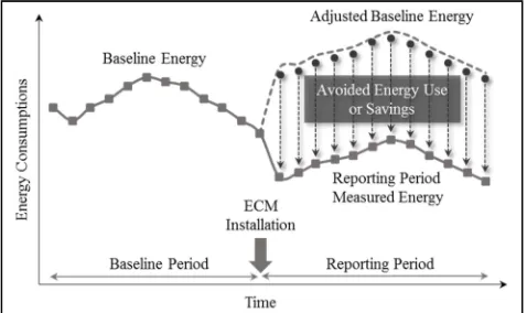
The absence of energy use can be computed by directly compared the energy use before and after implementation of an ECM which are currently practised. However, according to the IPMVP [12], the energy savings cannot be computed by simply comparing measurements of energy use before and after implementation of the ECM with the existence of variables that are affecting the energy use, such as weather, number of working days, occupancy or other factors. Fig. 1 illustrated the IPMVP framework in determining energy savings after implementation of ECM in the building.

Fig. 1 IPMVP Framework in determination of savings

In calculating savings, the impact of ECM on the energy use must be separated from the impact of the variables. So, baseline energy should be adjusted to the conditions of the reporting period. Then, the saving is the difference between adjusted baseline energy and reporting period measured energy. The savings can be calculated using Equation (1) below.

-(1)

where baseline energy use is the measured energy use prior to ECM and reporting energy use is the measured energy use after implementation of ECM. Routine adjustment is the factors that are routinely affecting energy use and has a trend while the non-routine adjustment is the energy governing factors non-routinely occur that affecting energy use during the reporting period. To properly report savings, the baseline period must be adjusted to the same set conditions of the reporting period. The adjustment terms in Equation (1) distinguish the proper savings report from a simple comparison before and after ECM implementation.

The IPMVP provide three different practices for quantifying energy savings and uncertainty levels from ECM namely as retrofit isolation, whole building measurement and calibrated simulation. This paper focused on energy savings for whole building measurement by applying option C from the protocol.

B. GUI Development

The Graphical User Interface (GUI) software is Windows Forms developed using Microsoft Visual Studio 2015 and SQL Server 2012 as the database storage. The programming language used for the software is Visual Basic code. This software is connected to Microsoft Excel for retrieving the outcomes of the simulations.

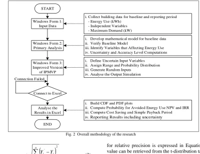
The GUI software is developed in [13], but the main purpose of that software is different with the GUI development in this study. The overall methodology for the development of Visual Basic GUI to quantify energy savings in an existing building using Monte Carlo simulations is illustrated in Fig. 2 and concisely described as below.

Windows Form 1: Primary Data Collection

The development of GUI starts with data collection of energy use and independent variables that have a significant correlation with the energy use. The building that was chosen as a case study in this paper has undergone multiple types of retrofitting programs which include replacing the CFL lighting system with T5 lighting technology, upgrading building control system with an energy monitoring system features and implementing chilled water treatment. The energy and variables data were collected for 12-months prior to retrofitting which is called as the baseline period and 12-months after retrofitting as reporting period.

1) Windows Form 2: Primary Analysis

In Windows Form 2, the mathematical model for baseline data is developed using regression technique to explore the correlation between the energy use and independent variable(s). This technique is implemented in [14] and [15] as well in order to assess the linear equation for multi-variable. Ke et al. [16] integrated multi-variable linear regression with Particle Swarm Optimization (PSO) algorithm to construct accurate baseline models. Authors in [17] developed a mathematical model for baseline data using inverse model. However, authors [13]–[15] is only focused on the development of the model, without any further analysis of energy saving and risk associated with the investment of the ECMs. The regression technique can be a single linear regression model which only considers an independent variable and multivariable linear regression model which considers more than one independent variables. The baseline model should meet the recommended values of R2 and CV-RMSE by IPMVP to ensure that the model would be able to predict the actual energy use in the building with a good accuracy. The R2 and CV-RMSE can be computed using Equation (2) and (3).

! Σ#ᵢ%ᵢ Σ#ᵢ Σ%ᵢ

(3)

where n is the number of observations, Yᵢ and Xᵢ is the dependent and independent variable for the n observations respectively.

START

Windows Form 1: Input Data

Windows Form 2: Primary Analysis

Windows Form 3: Improved Version

of IPMVP

Connect to Excel

i. Collect building data for baseline and reporting period - Energy Use (kWh)

- Independent Variables - Maximum Demand (kW)

i. Develop mathematical model for baseline data ii. Verify Baseline Model

iii. Identify Variables that Affecting Energy Use iv. Uncertainty and Accuracy Level Computations

i. Define Uncertain Input Variables ii. Assign Range and Probability Distribution iii. Generate Random Inputs

iv. Analyse the Output Simulation

Analyse the Results in Excel

i. Build CDF and PDF plots

ii. Compute Probability for Avoided Energy Use NPV and IRR iii. Compute Cost Saving and Simple Payback Period iv. Reporting Results including uncertainty

END Connection Failed

Fig. 2 Overall methodology of the research

where Yi' is the predicted value for energy use, Yi is the measured energy use, and Ῡ is the average measured energy. Degree of Freedom (DF) which is equal to n-p-1 is the number of observations minus the number of coefficient variables.

According to IPMVP, the R2 and CV-RMSE value should be greater or equal to 0.75 and less than 0.02 respectively.

The primary analysis continues with uncertainty and accuracy level computations. The measurement and modelling error are considered as the factors that contribute to the accuracy in quantifying energy savings. When a model is used to predict an energy for a given independent variable(s), the accuracy of the prediction is measured by standard error of the estimate. Thus, the standard error of estimate is calculated using Equation (4).

(

)

1 Error

Standard

2

1 '

− −

− =

∑

=

p n

Y Y n

i

i ₍₄₎

To justify the uncertainty in the M&V process, according to IPMVP, the savings must be larger than twice of the standard error of the estimate. For a proper savings report, energy savings should be presented in association with its precision and confidence level. Precision refers to error range within the true estimate value which is expected to occur with some specified level of confidence. The formula

for relative precision is expressed in Equation (5) where t value can be retrieved from the t-distribution table in statistic.

Relative Precision=t× √12×Standard Error

n-p-1 (5)

Windows Form 3: Monte Carlo Simulations

Monte Carlo simulations are a feasible alternatives technique when there are too many uncertain factors are involved in the computation of energy savings and to consider risk assessment in the analysis. It is crucial to assess the uncertainties in energy savings as well as to augment the decision-making process in the energy performance contracts (EPC). The details on how Monte Carlo simulations technique is utilised to quantify energy savings by incorporating risks in the financial assessment are described as below.

Define Uncertain Input Variable: The process begins with the identification of inputs that are subject to uncertain as listed below.

• Independent Variables: The potential influence of uncertainty in derived variable y for quantifying energy savings are due to the modelling and measurement errors present in the x’s from the mathematical models. • Investment cost: the investment expenditure for the

retrofitting programs, includes all the expenses for initial, additional or replacement equipment for measurement and verifications purpose.

• Annual cash flow: The annual cash flow is summations of all the in and out payments that take place during a year due to the initial investment. The cash in is the

(

)

1 1

2

1 '

− −

− =

−

∑

=

p n

Y Y

Y RMSE CV

n

i

(4)

value of annual cost savings after implementing retrofitting programs. The cash out is assumed to be zero due to the lack of information for the building study case.

• Discount rate: The discount rate is uncertain since the same amount of investment money at present has a different value in a few years into future. The annual cash flow in different years over the investment project period must be shifted to the same discount rate to have a comparable value.

Assign Range and Probability Distribution: The uncertain range of input variables are assumed to be normally distributed with its mean and standard deviation. Normal distribution provided the widest range of outcomes within the assigned range instead of fixed value.

Generate Random Inputs: The random inputs are generated within the assigning range and probability distributions. The generation of normal random numbers for input variables in this research is using Box-Muller method.

Analyse Output Simulation: The simulation iterates for 5,000 times resulting in a distribution of energy savings, NPV and IRR. The outcomes of the simulation are analyzed using Probability Density Function (PDF) and Cumulative Distribution Function (CDF) with confidence interval and summary statistics in Microsoft Excel. For PDF plot, the outputs data from the simulation are arranged with the high values clustered in the middle of the graph, and the rest are taper off symmetrically on both side of the graph. So, the estimation of the annual savings defined by the mean values which are in the middle of the plot and most likely to occur. The CDF is the probability of an observation output either above or below a specific value.

Analyse the Result in Microsoft Excel

The outputs of the simulation will be evaluated in term of probability including statistical confidence interval for energy savings, NPV and IRR. In addition, the cost savings and simple payback period are also computed. The savings is computed using Equation (1).

The formula of cost savings and simple payback period are expressed in Equation (6) and (7) respectively.

,

-./0 112 × 4 %56+ -89

%5+ -8: ; <

5=>

(6)

Payback Period= Investment Cost (RM)

Cost Savings (RM) (7)

Monte Carlo simulations are also used to analyse the NPV and IRR concerning the retrofitting performed in the building. NPV and IRR are used to explore the possible outcomes of financial assessment. It will estimate the future payments from a project and discounting them into the present value. The NPV can be calculated using Equation (8) as below.

@A . _{1 +}, _<

C

<=D

(8)

where Cn is the summation of cash flow for each period, n is the holding period, and r is discounted rate of return.

The profitability of an investment can be measured using an internal rate of return, IRR. An IRR is a discount rate that makes the NPV of all cash flows for a project equal to zero. It used the same formula as NPV. The value for IRR can be retrieved by setting the NPV equation to 0 and solve the discount rate, r.

III.RESULT AND DISCUSSION

The GUI software is executed in three different cases. In Case 1 and Case 2, single linear regression model is used, while Case 3 is performed using multi-variable linear regression model.

A. Case 1: Cooling Degree Days (CDD)

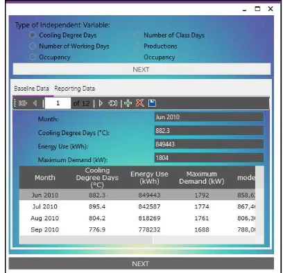
The monthly basis primary data such as energy use, CDD and maximum demand for both baseline and reporting period are gathered in Windows Form 1 as shown in Fig. 3. These data are extremely important in the development of appropriate baseline mathematical model for energy use in the building.

Fig. 3 Screenshot from windows form 1 for case 1 using proposed monte carlo simulations for M&V

(5)

The parameters for baseline mathematical model, uncertainty and accuracy level is automatically computed by the GUI software in Windows Form 2 once the user has keyed-in the primary data. The regression technique is used to develop baseline mathematical model. As can be seen in Fig. 4, the equation for baseline mathematical model is y = 670.01x + 267,478.53. From the observations, the R2 and CV-RMSE for this case are 0.82, and 0.0178 which comply with the IPMVP recommended values. The correlation of determination, R2 proved that energy use in the building is significantly affected by the CDD.

The set of random inputs are generated in Windows Form 3 after the required information namely number of iterations to be performed, investment cost and discount rate are entered by the user as shown in Fig. 5. Note that, the investment cost and discount rate are set to be RM450000 and 12% respectively for each case in this study.

Each case in this study is iteratively simulated for 5,000 times. The uncertain range of input variables is assumed to be normally distributed with its mean and standard deviation as tabulated in Appendix A.

The output simulations data is then passed to Microsoft Excel for further analysis using Probability Density Function (PDF) and Cumulative Distribution Function (CDF) with confidence interval and summary statistics.

Fig. 6 PDF and CDF plots for energy savings

Fig. 6 shows the bell curve of normal distribution for energy savings considering CDD as the independent variable retrieved for Microsoft Excel. From the mean value of PDF plot, the energy savings for the12-month periods after retrofitting is 230,993.2244 kWh. Hence, the cost savings and the simple payback period are RM 94,281.23 and 4.77 years respectively. The ranges for the twelve data points of energy savings at 95% level of confidence is 130,048.5954 kWh and 331,937.8533 kWh, which implies a relative precision of ±49.9%.

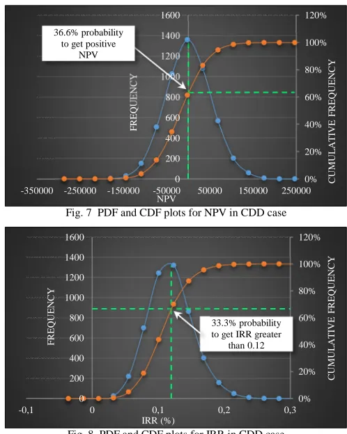
PDF and CDF plots in Fig. 7 and Fig. 8 are used to explore the possible outcomes of risk assessment in terms of NPV and IRR.

Fig. 7 PDF and CDF plots for NPV in CDD case

Fig. 8 PDF and CDF plots for IRR in CDD case

As for an IRR, it is seen that more than 30% probability of meeting an IRR greater than 12% as set earlier. Meanwhile, for an NPV, in this case, the project provides 36.6% probability of achieving positive NPV, thereby it indicates that the investment cost for this EE project is expected to be a profitable investment.

B. Case 2: Number Working Days (NWD)

In this case, the NWD is used as an independent variable to calculate energy savings. Like the case of CDD, the primary data for baseline and reporting period were first keyed-in by the user in Windows Form 1 as shown in Fig. 9.

The baseline primary data from Windows Form 1 are then used to develop a mathematical model for energy use in the building using regression method.

230993,2244 331937,8533 130048,5954 0% 20% 40% 60% 80% 100% 120% 0 200 400 600 800 1000 1200 1400 1600 1800

-100000 0 100000 200000 300000 400000 500000 600000

C U M U L A T IV E F R E Q U E N C Y F R E Q U E N C Y

ENERGY USE (KWH)

0% 20% 40% 60% 80% 100% 120% 0 200 400 600 800 1000 1200 1400 1600

-350000 -250000 -150000 -50000 50000 150000 250000

C U M U L A T IV E F R E Q U E N C Y F R E Q U E N C Y NPV 36.6% probability

to get positive NPV 0% 20% 40% 60% 80% 100% 120% 0 200 400 600 800 1000 1200 1400 1600

-0,1 0 0,1 0,2 0,3

C U M U L A T IV E F R E Q U E N C Y F R E Q U E N C Y IRR (%) 33.3% probability to get IRR greater

(6)

Fig. 9 Screenshot from windows form 1 for case 2 usingproposed monte carlo simulations for M&V

The baseline mathematical model describing the baseline data was found by regression technique to be y = 16,658.3x + 457,295.75. This baseline mathematical model is used to adjust baseline energy to the conditions of the reporting period. The model is assessed based on R2 and CV-RMSE parameters. The baseline data shows that the NWD has a significant effect on energy use in the building by having R2 and CV-RMSE of 0.79 and 0.0192 respectively, which meet the recommended values by IPMVP. The uncertainty and accuracy level of the baseline model are also computed as shown in Fig. 10.

Fig. 10 Screenshot from windows form 2 for case 2 using proposed monte carlo simulations for M&V

Fig. 11 shows the set random data generated using Monte Carlo simulations for the NWD case. The uncertain range of input variables is assumed to be normally distributed with its mean and standard deviation as tabulated in Appendix B.

The adjusted baseline is computed by substituting the random inputs into the baseline mathematical model.

Fig. 11 Screenshot from windows form 3 for case 2 using proposed monte carlo simulations for M&V

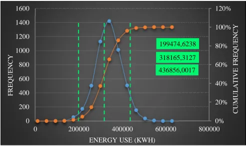
As shown in Fig. 12, the annual energy savings from the simulation is computed as 318,165.3127 kWh. The ranges of the energy savings at 95% confidence is 199,474.6238 kWh and 436,856.0017 kWh, which implies a relative precision of ±38.43%. By applying C1 tariff from TNB, the cost saving for NWD case is RM 126,099.04. The simple payback period of the investment cost is estimated to obtain within 3.57 years.

Fig. 12 PDF and CDF plots for estimation of savings for case 2

Fig. 13 PDF and CDF plots for NPV in NWD case

318165,3127 436856,0017 199474,6238

0% 20% 40% 60% 80% 100% 120%

0 200 400 600 800 1000 1200 1400 1600

0 200000 400000 600000 800000

C

U

M

U

L

A

T

IV

E

F

R

E

Q

U

E

N

C

Y

F

R

E

Q

U

E

N

C

Y

ENERGY USE (KWH)

0% 20% 40% 60% 80% 100% 120%

0 200 400 600 800 1000 1200 1400

-250000 -150000 -50000 50000 150000 250000 350000 450000

C

U

M

U

L

A

T

IV

E

F

R

E

Q

U

E

N

C

Y

F

R

E

Q

U

E

N

C

Y

NPV

97.7% probability to get

(7)

From Fig. 13, the NPV of a 7-years investment period is RM 78,925.14 whilst from the CDF plot, the probability to get a positive value of NPV is 97.7%. With the high probability of getting NPV greater than 0, this retrofitting project is expected to gain profit within the project period.

Based on the IRR plot in Fig. 14, there is almost 100% probability of achieving an IRR greater than 12% which results in a profitable investment over the project period.

Fig. 14 PDF and CDF plots for IRR in NWD case

C. Case 3: Multi-Variable

Fig. 15 below shows the Windows Form 1 for the multi-variable case combining CDD and NWD. The analysis was performed using multivariable linear regression technique.

The primary data such as energy use, CDD, NWD and maximum demand for baseline and reporting period are keyed-in by the users in Windows Form 1 as can be seen in the figure above.

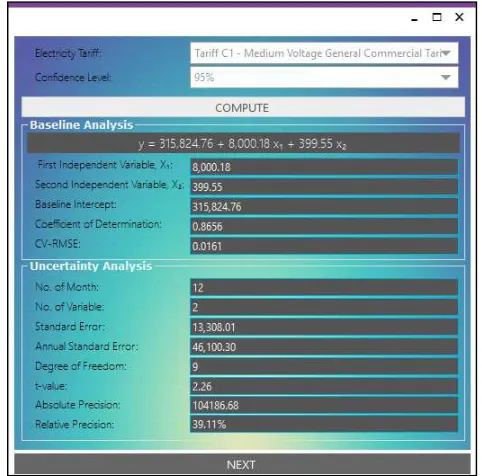
For a baseline of 12 monthly energy use, CDD and NWD data points, the derived baseline mathematical model using regression technique is y = 8000.18x1 + 399.55x2

+315,824.76. The 12-months baseline data of the multi-variable shows a better correlation between energy use in the building. This is confirmed by the values of R2, i.e., 0.8656

and CV-RMSE of 0.0161. On the other hand, the uncertainty and accuracy level of the baseline model is also computed as shown in Fig. 16.

It can be seen in Fig. 17 the set of random data generated using Monte Carlo simulations for the multi-variable case after the required information such as a number of iterations, investment cost, and discount rate are entered by the users. The uncertain range of input variables are assumed to be normally distributed with its mean and standard deviation as illustrates in Appendix C. The adjusted baseline is computed by substituting the random inputs into the baseline mathematical model. The investment cost and discount rate for this case are also set to be RM450000 and 12% respectively.

0% 20% 40% 60% 80% 100% 120%

0 200 400 600 800 1000 1200 1400 1600 1800

0 0,1 0,2 0,3 0,4

C

U

M

U

L

A

T

IV

E

F

R

E

Q

U

E

N

C

Y

F

R

E

Q

U

E

N

C

Y

IRR (%)

99.2% probability to get IRR greater than

(8)

The output simulations data is then passed to Microsoft Excel for further analysis using Probability Density Function (PDF) and Cumulative Distribution Function (CDF) with confidence interval and summary statistics.

The annual energy savings obtained from the Monte Carlo simulations in this case of multivariable is 267,424.52 kWh as plotted in Fig. 18. The range of the savings at 95% confidence is computed between 183,726.0138 kWh to 351,123.0332 kWh, which implies a relative precision of ±39.11%. The cost savings is RM 107,578.65 and the simple payback period of the investment cost is estimated to obtain within 4.18 years.

Fig. 18 PDF and CDF plots for estimation of savings for case 3

In the multi-variable case, the probability to get NPV greater than 0 is 74.5% as shown in Fig. 19. With the high probability of getting NPV greater than 0, it informs the investors that the investment of the project is a profitable investment.

Fig. 19 PDF and CDF plots of NPV for case 3

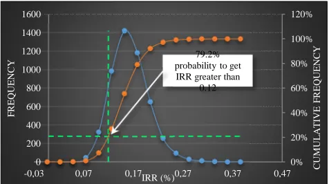
Based on the IRR plot in Fig. 20, the probability of achieving an IRR greater than 12% is 79.2% which results in a profitable investment over the 7-years project period.

Fig. 20 PDF and CDF plots of IRR for case 3

From the analysis, the case 3 with multivariable linear regression model provides a better correlation than single linear regression as in case 1 and case 2 for both R2 and CV-RMSE indicators. Thus, it shows that more than one variable is affecting the energy use in the building.

From the findings, the multiple linear regression is also a better model by having a smaller value of standard error. It can be specified in this case; the multivariable linear regression model provides a better accuracy than the single linear regression model.

For the cost savings, TNB tariff C1 is used in the calculation. By assuming the investment cost of RM 450,000, the analyses show a payback period within 3 to 5 years to repay the total initial investment cost from the energy savings.

IV.CONCLUSIONS

In this paper, a new M&V framework with risk assessment is developed using Monte Carlo simulations. It was developed using Visual Basic GUI with multiple Windows Forms, and the results are analysed in Excel template. The GUI has been tested with three different cases, 1) Cooling Degree Days (CDD), 2) Number of Working Days (NWD) and 3) Multi-variable that combining CDD and NWD using single linear regression model and multi-variable linear regression model. From the case studies, the multi-variable model seems to be more accurate with higher precision level.

The Monte Carlo simulations based M&V technique presented in this paper earns an additional point in its ability to provide a better view of investment risks from the distribution of NPV and IRR and probability of getting the required profitability.

ACKNOWLEDGMENT

We would like to thank Malaysia Ministry of Education and Universiti Teknologi MARA (UiTM) who have sponsored this paper under Research Acculturation Grant Scheme (RAGS), 600- RMI/RAGS 5/3 (194/2014).

REFERENCES

[1] L. F. Cabeza, D. Urge-Vorsatz, M. A. McNeil, C. Barreneche, and S. Serrano, “Investigating greenhouse challenge from growing trends of electricity consumption through home appliances in buildings,”

Renew. Sustain. Energy Rev., vol. 36, no. August, pp. 188–193, 2014.

[2] U.S. Energy Information Administration, International Energy

Outlook 2016, vol. 0484(2016), no. May 2016. 2016.

[3] J. S. Hassan, R. M. Zin, M. Z. A. Majid, S. Balubaid, and M. R. Hainin, “Building energy consumption in Malaysia: An overview,” J.

Teknol., vol. 70, no. 7, pp. 33–38, 2014.

[4] Economic Planning Unit Prime Minister’s Department Malaysia, “Sustainable Usage of Energy to Support Growth,” 2015.

[5] F. Version, “Malaysian Industrial Energy Efficiency Improvement Project ( MIEEIP ) Government of Malaysia United Nations Development Programme Global Environment Facility,” no. January, 2008.

[6] N. S. Razali and N. Y. Dahlan, “Whole Facility Measurement for Quantifying Energy Saving in an Office Building , Malaysia,” vol. 785, no. Cdd, pp. 676–681, 2015.

[7] S. Mohd Aris, N. Y. Dahlan, M. N. Mohd Nawi, T. A. N. Tengku Putra, and M. Z. Tahir, “Quantifying Energy Savings for Retrofit Centralized HVAC System at Selangor State Secretary Complex,” vol. 5, no. cdd, pp. 93–100, 2015.

[8] F. M. A. Rahman, N. Y. Dahlan, and N. S. Razali, “Modelling Adjusted Baseline Energy in an Office Building using Artificial

351123,0332 183726,0138 267424,5235 0% 20% 40% 60% 80% 100% 120% 0 200 400 600 800 1000 1200 1400

0 100000 200000 300000 400000 500000

C U M U L A T IV E F R E Q U E N C Y F R E Q U E N C Y

ENERGY USE (KWH)

0% 20% 40% 60% 80% 100% 120% 0 200 400 600 800 1000 1200 1400

-300000-200000-100000 0 100000 200000 300000 400000 500000 _CU

M U L A T IV E F R E Q U E N C Y F R E Q U E N C Y NPV (RM) 74.5% probability to get

positive NPV 0% 20% 40% 60% 80% 100% 120% 0 200 400 600 800 1000 1200 1400 1600

-0,03 0,07 0,17 0,27 0,37 0,47 C

U M U L A T IV E F R E Q U E N C Y F R E Q U E N C Y IRR (%) 79.2% probability to get IRR greater than

(9)

Neural Network,” vol. 785, pp. 655–660, 2015.

[9] E. Mills, S. Kromer, G. Weiss, and P. A. Mathew, “From volatility to value: Analysing and managing financial and performance risk in energy savings projects,” Energy Policy, vol. 34, no. 2 SPEC. ISS., pp. 188–199, 2006.

[10] J. Jackson, “Promoting energy efficiency investments with risk management decision tools,” Energy Policy, vol. 38, no. 8, pp. 3865– 3873, 2010.

[11] P. Lee, P. T. I. Lam, F. W. H. Yik, and E. H. W. Chan, “Probabilistic risk assessment of the energy saving shortfall in energy performance contracting projects-A case study,” Energy Build., vol. 66, pp. 353– 363, 2013.

[12] EVO, “International Performance Measurement and Verification Protocol,” vol. 1, no. January, 2012.

[13] A. M. T. Jr and A. R. Ligisan, “Development of PHilMech Computer Vision System ( CVS ) for Quality Analysis of Rice and Corn,” vol. 6, no. 6, pp. 1060–1066, 2016.

[14] R. Jing, M. Wang, R. Zhang, N. Li, and Y. Zhao, “A Study on Energy Performance of 30 Commercial Office Buildings in Hong Kong,” Energy Build., vol. 144, pp. 117–128, 2017.

[15] M. R. Abdullah, A. B. H. M. Maliki, R. M. Musa, N. A. Kosni, and H. Juahir, “Intelligent Prediction of Soccer Technical Skill on Youth Soccer Player’s Relative Performance Using Multivariate Analysis and Artificial Neural Network Techniques,” Int. J. Adv. Sci. Eng. Inf.

Technol., vol. 6, no. 5, pp. 668–674, 2016.

[16] M.-T. Ke, C.-H. Yeh, and C.-J. Su, “Cloud computing platform for real-time measurement and verification of energy performance,” Appl.

Energy, vol. 188, pp. 497–507, 2017.

[17] J.-H. Ko, D.-S. Kong, and J.-H. Huh, “Baseline Building Energy Modeling of Cluster Inverse Model by using Daily Energy Consumption in Office Buildings,” Energy Build., vol. 140, pp. 317– 323, 2017.

APPENDIX A

Parameters Mean Standard Deviation

Cooling Degree Days, (°C)

831.5

22.11811269 837.1

840.9 820.4 865.3 809.3 820.7 827.7 775.9 821.2 800.8 831.2 Investment Cost

(RM) 450000 45000

Revenue (RM) 94281.22689 9428.122689

Discount Rate 12% 0.024

APPENDIX B

Number of Working Days

(Day)