A Comparative Study between Ridit and Modified Ridit Analysis

Published online December 10, 2013 (http://www.sciencepublishinggroup.com/j/ajtas) doi: 10.11648/j.ajtas.20130206.23

A comparative study between ridit and modified ridit

analysis

Ebuh Godday Uwawunkonye, Oyeka Ikewelugo Cyprian Anaene

Department of Statistics, Faculty of Physical Sciences, Nnamdi Azikiwe University, Nigeria

Email address:

[email protected] (Ebuh G.U.)

To cite this article:

Ebuh Godday Uwawunkonye, Oyeka Ikewelugo Cyprian Anaene. A Comparative Study between Ridit and Modified Ridit Analysis. American Journal of Theoretical and Applied Statistics. Vol. 2, No. 6, 2013, pp. 248-254. doi: 10.11648/j.ajtas.20130206.23

Abstract:

This paper compares ridit analysis with modified ridit analysis. The comparison was then illustrated with an example. It was observed from the example at least, that when the sample sizes of the two samples being compared are too disparate, a more reliable conclusion using the Bross ridit analysis is likely to be reached only when the group with the larger sample size is used as the reference group. Otherwise Bross ridit analysis would lead to conflicting conclusions, depending on which group is used as the reference group. Modified ridit analysis treats the groups being studied as samples drawn from some larger populations in which the variances or standard deviations as well as the results obtained are the same no matter which sample is used as the reference group. The modified procedure is therefore preferable to ridit analysis especially in cases where the groups being compared are samples from some populations.

Keywords:

Samples Estimates, Populations, Bross Mean Ridit, Chi-Square, Significance

1. Introduction

Suppose that we have sample data drawn from a number of populations each of which is assumed to have in-built qualitatively ordered categories or classes. For example suppose we have random samples of patients by age say of a certain disease whose condition is ordered from critical to severe, poor, improved, most improved, etc. In an automobile accident involving some passengers, a passenger’s level of injury may range from none through mild, severe to fatal.

Although these graduations may be coarse, discrete and still finite, they are never-the-less more descriptive and exhaustive than merely using some dichotomous classifications such as none or all, yes or no, present or absent, etc, which are fairly crude and not fully descriptive.

To compare these samples and reach clear conclusion is often difficult. However in the above and similar cases, the grading of the degree of seriousness is subjective and may not be reliable. Furthermore, it is difficult to find a readily interpretable summary index for such a data-set and to make comparisons among different samples in an intelligent way. The conventional chi-square analysis may be performed, but important information on the natural ordering of the categories would be lost.

A frequently employed procedure is to number the categories from say, 0 for the least serious to some highest

number for the most serious, calculate means and standard deviations, and then apply the‘t’ test or analysis of variance. There is however also a problem with this approach. The assignment of ordered numerical codes with equal spacing to the various categories of the variable under study is often arbitrary. It is a device that defines a metric on the categories of a qualitative variable which may or may not represent the true pattern of relationships among these categories.

A technique that does not attempt to quantify the categories but rather works with their natural ordering is the ridit analysis developed by Bross(1958).

The term ridit is an acronym for ‘relative to an identified distribution’ of the proportions or frequencies over the various ordered categories of some chosen standard or reference population, ‘relative’, in the sense that the proportions or frequencies of occurrence of observations in the various ordered categories of a population of interest, are compared with the proportions or frequencies in the corresponding ordered categories of the reference population or group. Virtually the only assumption made in ridit analysis is that the discrete categories represent intervals of an underlying but unobservable continuous distribution. No assumption is made about normality or any other form for the distribution.

2. Ridit Analysis

Ridit analysis begins with the selection of one of the groups of data with the specified ordered categories to serve as a standard or reference population for the other groups, often referred to as comparison groups. Having selected a reference group or population, one then calculates a ‘ridit’ or score for each of its categories. The score or ridit for a given category is calculated as the cumulative frequency of all the categories lower in degree of seriousness than the category of interest plus one-half of the frequency for that category, all divided by the total frequency or the population size of the reference group. Thus using the data in the form of frequencies shown in table 1, the ridit for a category of the reference population is the proportion of all subjects or observations from the reference group falling in the lower ranking categories plus half the population falling in the given category

2.1. Methodology

Table 1: Data Format for Ridit Analysis GROUPS

Ordered category of criterion variable (Ci)

Y (Reference, fiy)

X (Comparison, fix)

Total (tixy)

C1 f1y fix tixy(=fix+fiy)

C2 f2y f2x t2xy(=f2x+f2y)

. . . .

. . . .

. . . .

Ck fky fkx tkxy(=fkx+fky)

Total ny nx nx+ny

Once the ridits for all the categories of the reference population are determined, they are taken as values of a dependent variable for the other groups. Given the distribution of any other group over the same categories the mean ridit for that group may be calculated. It is simply the sum of the products of observed frequencies, times the ridits obtained from the reference population for the corresponding categories divided by the total frequency for that group.

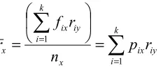
Thus using the frequencies in Table 1, the ridit of the ith category of the reference population Y is

∑

∑

₋

= −

=



₌

₊















+

=

1

1 1

1 i

j

iy jy y

i

j

iy jy

iy

p

p

n

f

f

r

(1)

Where

_p

jy

and

_p

iy

are respectively the proportions of the

total observations in the jth and ith categories of the reference population Y for j = 1, 2 . . . i-1, i = 1, 2 … k. The mean ridits

r

_x for any other group X is then calculated as

∑

∑

=

=

₌













=

k

i iy ix x

k

i iy ix

x

p

r

n

r

f

r

1

1 (2)

where

_P

ixis the proportion of cases in, or the relative frequency of the ith category of group or population X, for i = 1, 2. . . k. The mean ridit for the reference population Y is by the definitions in equations 1-2 always equal to 0.50. This means that if any two subjects are selected at random from the reference population Y, then one of them would be expected to experience a more serious condition on the criterion variable half of the time, and a less serious condition also half of the time than the others subject in the reference population.

The mean ridit for any other group X, is interpreted as follows; Given the reference group Y and any other group X, then the mean ridit

r

_x for the comparison group X is an estimate of P(X ≥ Y), that is of the probability that a randomly selected subject from group X, the comparison group, has a condition that is at least as serious as that of a randomly selected subject from group Y the reference group on the criterion variable. Thus if the mean ridit

r

_x for a given comparison group X is more than 0.50, then more than half of the time or randomly selected subject from it will have a more serious condition than a randomly selected subject from the reference group Y. If on the other hand the ridit for the group is less than 0.50, we would conclude that a randomly selected subject from it would be expected to experience a less serious condition than a randomly selected subject from the reference group Y. A mean ridit of 0.50 for any group would imply that subjects from that group would tend to experience neither more nor less serious condition than subjects from the reference group.

Therefore if Rx is the mean ridit of a comparison

population X from which a random sample of size nx has

been drawn to obtain

r

_x, then a null hypothesis that needs to be tested is

H0: Rx ≥ 0.50, versus Hi: Rx ≤ 0.50 (3)

Where 0.50 is the mean ridit of the standard or reference population Y.

It has been shown by Bross(1958) that for sufficiently large sample size nx,

r

_x is approximately normally

distributed with mean Rx and variance

( )

x x

n

r

Var

12

1

=

(4)

Hence the null hypothesis of Eqn 3 may be tested using the test statistic.

(

)

( )

(

)

2

2 2

50

.

0

12

50

.

0

−

=

−

=

x x

x x

r

n

r

Var

r

Which has approximately a chi-square distribution with 1 degree of freedom for sufficiently large

_n

x . Ho is rejected at the α level of significance if

2 1 ; 1 2

α

χ

χ

≥

− (6)

Otherwise H0 is accepted.

2.2. Illustrative Example 1

The data of Table 2 shows the degree of the effects of the concentration of some poisonous chemical on the blood stream of three groups of employees by work place.

Table 2: Distribution of Employees by work place and level of reaction of some poisonous chemical

Work place

Reaction to poisoning (severity of condition)

A(Y) B(X) C(Z)

Total

Txy Tyz Txz

None 35 58 24 93 59 82

Moderate 31 392 126 423 157 182

Severe 17 96 39 113 56 135

Critical 8 21 29 29 37 50

Fatal 14 48 24 62 38 72

Total 105(=ny) 615(=nx) 242(nz) 720 347 523 It can be seen from Table 2 that groups Y and X have a sample size ratio of approximately 1:6, groups Y and Z, a sample size ratio of approximately 1:2 and groups X and Z a sample size ratio of approximately 3:1. To find out the effect different sample sizes have on ridit analysis, we have use each of the groups or populations X, Y and Z alternatively as the comparison and reference populations.

First using Y(A) as the reference group we calculate the ridits for the categories of Y from Table 2 using Equation 1 as

None :

₀

_.

₁₆₇

_;

105

20

35

1y

=

=

r

Moderate:

₀

_.

₄₈₁

_;

105

2

31

35

2

=

+

=

y

r

Severe:

₀

_.

₇₁₀

_;

105

2

17

31

35

3

=

+

+

=

y

r

Critical:

₀

_.

₈₂₉

_;

105

2

8

17

31

35

4

=

+

+

+

=

y

r

Fatal:

₀

_.

₉₃₃

_;

105

2

14

8

17

31

35

5

=

+

+

+

+

=

y

r

From the ridit scores we calculate the mean ridit for X(B) Equation 2 as

( )(

58 0.167

) ( )(

392 0.481

) ( )(

96 0.710

) ( )(

21 0.829

) ( )(

48 0.933

)

615

x

r= + + + +

328.5316 0.534 615

x

r = =

Thus the ridit analysis estimates that the probability is 0.534 that a randomly selected employee in work place B(X) has as serious or more serious reaction to the chemical poisoning than a randomly selected employee in work place A(Y), the reference group.

The corresponding variance is from Equation 4

( )

_{( )}

0

.

0001

7380

1

615

12

1

₌

₌

=

x

r

Var

Hence the test statistic for the null hypothesis of Equation 3 is

(

)

₁₁

_.

₅₆

0001

.

0

50

.

0

534

.

0

2

2

=

−

=

χ

which with 1 degree of freedom is highly statistically significant.

A similar calculation may be made for work place C(Z) as a comparison group again using work place A(Y) as the reference group yielding an estimated mean ridit.

From Equation 2 as

573

.

0

242

7059

.

138

=

=

z

r

with a variance of

( )

_{( )}

0.0003

242 12

1

= =

z

r Var

Hence the corresponding chi-square test statistics is

(

)

₁₇

_.

₇₆₃

0003

.

0

0053

.

0

0003

.

0

50

.

0

573

.

0

2

2

=

−

=

=

χ

which is again highly statistically significant.

If instead work place B(X) has been used as the reference group or population the ridit scores for X would be

Mild:

0

.

047

;

615

2

58

1x

=

=

r

Moderate:

₀

_.

₄₁₃

_;

615

2

392

58

2

=

+

=

x

r

Severe:

₀

_.

₈₁₀

_;

615

2

96

392

58

3

=

+

+

=

x

r

Critical:

₀

_.

₉₀₅

_;

615

2

21

96

392

58

4

=

+

+

+

=

x

r

Fatal:

0

.

961

615

2

48

21

96

392

58

5

=

+

+

+

+

=

x

r

Using these values in Equation 2 we calculate the mean ridit for work place A(Y), now treated as a comparison

group as

₀

_.

₄₆₆

105

915

.

48

₌

=

This value is simply equal to

1

−

r

_x which is meaningfully reflecting the fact that a complementary probability is being estimated. The variance of this mean ridit from Equation 4 is

( )

0

.

0008

105

12

1

)

(

r

y

=

=

Var

The corresponding chi-square test statistics is

(

)

₁

_.

₄₄₅

0008

.

0

50

.

0

466

.

0

2

2

=

−

=

χ

which is not significant at the 5% significance level. Thus the change in choice of the reference group or population has resulted in a non significant effect. In other words, if we had used work place B(X) as the reference group or population instead of work place A(Y) we would conclude that employees in work place A(Y) now treated as the comparison group are as seriously affected by the chemical poisoning as the employees in work place B(X). But if we had used workplace A(Y) as the reference group we would conclude that employees in workplace B(X) are more seriously affected by the chemical poisoning than the employees in workplace A(Y).

Hence conclusions reached using ridit analysis often depend on which group is used as a reference group or population, and which is used as a comparison group.

We now present a modified method of estimating ridits that are independent of which populations are used as reference and which as comparison groups.

3. Modified Ridit Analysis

Implicit in the Bross ridit procedure is the assumption that the reference group is a population. Although the author did mention the difficulty of selecting an appropriate reference group, he failed to explicitly suggest an appropriate procedure when either of the two groups to be compared might serve as a reference group. The main cause of the problem with the Bross procedure is in the difficulty of determining an appropriate standard deviation to use in the denominator of the test statistic. Interchanging the reference and comparison groups merely interchanges the roles of these groups, while the mean ridits estimated are still meaningful and useful probabilities. However, if the sizes of the two groups that are being compared are very different using one of the groups rather than the other as a reference group affects the standard deviation and hence result of the test. Furthermore, if all available groups are regarded as samples from their respective populations, an additional source of variability is also introduced, since the ridit scores are then subject to variations themselves.

The results of the following procedure are similar to those of ridit analysis in interpretation but the procedure makes the explicit assumption that all the groups are to be regarded as samples from their respective populations. The method is based on Mann and Whitney (1947). Area works by Conover (1973) and Oyeka (1992) provide theoretical bases. Other researches include Mieke etal (2009), Pouplard etal (1997), and Rao and Caliguin (1993).

3.1. Methodology

Let

y

y

n j

j(=1,2,....,)be a set of ny observations made on group

or population Y (Bross reference group), occurring with frequencies, f_1y , f_2y … f_ky across c1, c2 ... ck the k

categories of a criterion variable such that

∑

=

=

k

i i

y

f

y

n

1

.

Similarly let

_x

x n i

i(=1,2,....,)be a set of nx observations made on

any other group or population X referred to as the comparison group occurring with frequencies f_1x, f2x ... .

kx

f respectively across the k categories of the same

criterion variable, such that

∑

=

= k

i i x fx

n

1

The data format is as in Table 1

Now for the reference group Y and any comparison group X define the function uij as











<

−

=

>

=

j i

j i

j i ij

y

x

if

y

x

if

y

x

if

u

,

1

,

0

,

1

(7)

for i = 1, 2 . . . . nx; j = 1, 2 ... ny

Let

(

1

)

:

(

0

)

:

(

1

)

0

−

=

=

=

=

=

=

−

+

ij ij

ij

x

P

u

x

P

u

u

P

π

π

π

(8)

Where

1

0

=

+

+

−

+

x

x

x

π

π

π

(9)

Also define

∑ ∑

= =

=

nx y

i n

j ij

x

u

W

1 1

(10)

Now

( )

( )

2

; 

  

 

− − + = −

= + x − xVaru + x − x +x − x u

E _ij

π

π

_ij

π

π

π

π

(11)

Also

( )

∑ ∑

( )

= =

=

nx y

i n

j ij

x

E

u

W

E

1 1

OR

( )













₋

=

n

n

+

x

−

x

W

E

_{x x y}

π

π

(12)

Note that x

+

π

, x

0

π

and x

−

probabilities that a randomly selected subject from the comparison population X is in a more serious, as serious as or less serious condition on the criterion variable than a randomly selected subject from the reference population Y. In terms of Bross mean ridit

x x x x x x

r

r

0 _ 0

2

1

1

;

2

1

π

π

π

π

+

−

=

+

=

+ (13)

These probabilities are estimated as functions of 0

,

_x

x

f

f

+ and

f

_x− where

f

_x+

,

f

_x0 and

f

_x− are respectively the number, or frequencies of occurrence, of 1’s 0’s and -1’s in the frequency distribution of the nxny

values of these numbers in uij, i = 1, 2 … nx; j = 1, 2 … ny.

The sample estimates of x x

− +

−

π

π

, the difference

between x

+

π

and x

−

π

is from equation 12

y x x x y x x x x

n

n

f

f

n

n

W

+ −

−

+

₋

=

=

−

π

π

⌢

₍₁₄₎

Also the sample estimate of the variance of

w

_x is obtained using equation 13 as

n

n

w

n

n

y x x x x y x x w Var 2 ˆ ˆ ) ( −      ₋ + +

=

_π

_π

(15)

Hence the sample estimate of x

0

π

is

y x x x

n

n

f

0 0ˆ

=

π

(16)

Also it is easy to show using equations 9 and 14 that the

estimated values of x

+

π

and x

−

π

are respectively

(

)

















₋

+

−

=

















+

−

=

+ − + y x x x y x x y x x x x

n

n

f

f

n

n

f

n

n

W

0 2 1 0ˆ 2 1 ˆ

1

1

π

π

(17) And

(

)

















₋

−

−

=

















−

−

=

+ − − y x x x y x x y x x x x

n

n

f

f

n

n

f

n

n

W

0 2 1 0ˆ 2 1 ˆ

1

1

π

π

(18)

It has been shown by Hajek (1969) and Conover (1973) that the variance of

W

x is estimated as

( )

(

)

₍

(

_{) (}

)

₎

            + − + − − + + =

∑

= y x y x k i ixy ixy y x y x x n n n n t t n n n n W

Var 1 ₃

3

1 3

1

(19)

that a randomly selected subject from the comparison population Xi is in a more serious condition on the criterion

variable than a randomly selected subject from the reference population Y and the probability that the randomly selected subject is in a less serious condition, provides a measure of the relative seriousness of the condition in the populations. Now if population X and population Y are in fact the same population, then the relative difference between the probabilities of seriousness of the condition in the two populations would be = Zero, so

that

−

=

0

− +

x x

π

π

Hence a more general null hypothesis that needs to be tested here is

H0:

0

δ

π

π

+x

−

−x

≥

versus H1:

(

1

1

)

,

₀

0

−

<

<

<

−

− +

δ

δ

π

π

x x (20)

Now for sufficiently large nx and ny, Wx has

approximately the normal distribution with mean E(Wx) of

equation 12 and variance, Var(Wx) of equation 19.

Hence the null hypothesis of equation 20 may be tested using the test statistic

( )

(

)

( )

x x x

W

Var

W

E

W

2

2

₌

−

χ

(21)

OR

(

)

( )

x

y x x W Var n n

W 0 2

2

δ

χ

= − (22)

Which has approximately a chi-square distribution with 1 degree of freedom for sufficiently large nx, ny where

Var(Wx) is given in equation 19. H0 is rejected at the α

level of significance if Equation 6 is satisfied. Otherwise H0 is accepted.

3.2. Illustrative Example 2

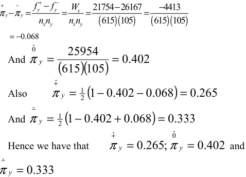
Let us now use the modified method to re-analyze the data in Table 2 earlier used to illustrate ridit analysis in example 2. We first use work place A(Y) as the reference population and work place B(X) as the comparison population

Now from equation 13 and Table 2, we have that

( )( ) ( )(

392 35 96 35 31

) ( )(

21 35 31 17

) ( )(

48 35 31 17 8

)

x

f+= + + + + + + + + +

26167

=

Also

( )(

58 31 17 8 14

) ( )(

392 17 8 14

) ( )(

26 8 14

) ( )( )

21 14

x

f−= + + + + + + + + +

21754

=

And f_x0=

( )( ) ( )( ) ( )( ) ( )( ) ( )( )

58 35+ 392 31+ 96 17+21 8 +48 14

25954

=

068

.

0

64575

4413

ˆ ˆ

=

=

−

−

+

x x

π

π

Also from equation 3.13

( )( )

0.402 105

615 25954 0ˆ

= =

x π

From equation 17

(

1

0

.

402

0

.

068

)

0

.

333

2

1 ˆ

=

+

−

=

+

x

π

And from equation 18

(

1

0

.

402

0

.

068

)

0

.

265

2 1 ˆ

=

+

−

=

−

x

π

Therefore the estimated probabilities are

265

.

0

402

.

0

;

333

.

0

ˆ

0ˆ ˆ

=

=

=

−

+

x x

x

π

and

π

π

Hence the modified approach estimates that the probability is 0.333 that a randomly selected employee in work place B(X) (the comparison population) is more seriously affected by the chemical poisoning than a randomly selected employee in work place A(Y) (the reference population) 0.402 that the employee is as seriously affected and 0.265 that the employee is less seriously affected.

Notice that as earlier obtained using Gross mean ridit

(

0

.

402

)

0

.

534

333

.

0

+

1₂

=

=

x

r

The fact that the probability of experiencing equal severity of condition has now been estimated separately is an important and useful additional information and advantage of the modified method over Bross ridit analysis.

The variance of Wx is estimated from equation 19 as

( ) ( )( )( )615 105 721 78196218

1 12, 268,144

3 373247000

x

Var W = _ − _=

 

The null hypothesis of Equation 20 (with

δ

₀

=

0

) may now be tested using the test statistic

(

)

_1.587

268144 , 12

474569 , 19 144 , 268 , 12

0

4413 2

2₌ − _{= =}

χ

which with 1 degree of freedom is not statistically significant. If we now interchange the roles of Y and X, that is if X now becomes the reference group and Y, becomes the comparison group, we would have that

∑

∑

=

−

= +













=

k

j

i

i i j

y

f

y

f

x

f

2

1

1

( ) ( ) ( ) ( )

31 58 17 58 392 8 58 392 96 14 58 392 96 21

= + + + + + + + + +

26167

=

And

1

2 1

k k

y j i

j i j

f f y f x

− −

= = +

 

=  

 

∑

∑

=

( ) ( ) ( ) ( )

35 392 96 21 48+ + + +31 96 21 48+ + +17 21 48+ +8 48 21754

=

Also

25954

1

0

=

∑

=

=

k

i i i y

f

yf

x

f

as before

Therefore,

( )( ) ( )( )

21754 26167 4413

615 105 615 105

y y x

y y

x y x y

f f W

n n n n

π π+ − =− +− −= = − = −

0.068

= −

And

( )( )

0

.

402

105

615

25954

0ˆ

=

=

y

π

Also ₂1

(

1

0

.

402

0

.

068

)

0

.

265

ˆ

=

−

−

=

+

y

π

And −ˆ

=

1₂

(

1

−

0

.

402

+

0

.

068

)

=

0

.

333

y

π

Hence we have that

0

.

265

;

0

.

402

0ˆ ˆ

=

=

+

y

y

π

π

and

333

.

0

ˆ

=

−

y

π

These are the same values obtained when work place A(Y) is used as the reference population and work place B(X) is used as the comparison population. Hence the value of the estimated variance of Wy remains the same as that of

Wx and the value of the test statistic and the attained

significance level remain unchanged. Hence the same conclusions are reached with the modified ridit analysis irrespective of which of the populations is used as the reference group and which as the comparison group.

Thus the only changes that result when the roles of the two groups are interchanged are that the sign of W changes;

x

+

π

is interchanged with y

−

π

and x

−

π

is interchanged

with y

+

π

, unlike is the case with Bross ridit analysis. Table 3 shows the results of the analysis of the data in Table 2 by both the ridit analysis and the modified ridit analysis using each of the work places in turn as the reference group or population

4. Results and Discussions

The chi-square test statistics of Equation 5 and 22 may be expressed in terms of unit-normal z-scores and are hence so reported in Table 3 as can be seen from this table, interchanging the reference and comparison groups has a marked effect on the Bross analysis, often changing the attained significance level drastically. In modified ridit analysis no such effect is observed. Here the variance (standard deviations) and the attained significance levels remain the same when the reference and comparison groups are interchanged. Furthermore the significance levels attained by the Bross ridit analysis appear to be generally lower than those by the modified ridit analysis. In fact it is only when the same size of the reference group is very large, as in group X, that the significance levels attained by the two procedures are approximately the same.

used as the reference group. With the modified ridit analysis on the other hand, no such problem is encountered. Furthermore when the difference between the sample sizes of the groups being compared, is not too large, as in the

case of groups X and Z, the attained levels of significance seem to suggest that the modified procedure would still be the preferred method in terms of consistency of conclusions.

Table 3: Comparison of two Ridits methods

Data Ridit Analysis Modified Ridit Analysis

Set

r

S Z p-value

+ˆ

π

π

0ˆ

π

−ˆ S Z P-value

Workplace A(Y) as reference group

Workplace B(X) 0.534 0.012 2.83 0.005 0.333 0.402 0.265 3502.60 1.26 0.208

Workplace C(Z) 0.573 0.019 3.84 0.00 0.456 0.235 0.309 1624.89 2.29 0.022

Workplace B(X) as reference group

Workplace A(Y) 0.466 0.028 -1.21 0.226 0.265 0.402 0.333 3502.60 -1.26 0.208

Workplace C(Z) 0.554 0.019 2.84 0.005 0.365 0.378 0.257 5738.39 2.80 0.005

Workplace C(Z) as reference group

Workplace A(Y) 0.427 0.028 -2.61 0.009 0.309 0.235 0.456 1624.89 -2.29 0.022

Workplace B(X) 0.448 0.012 -4.33 0.000 0.257 0.378 0.365 5738.35 -2.80 0.005

5. Conclusion

Modified ridit analysis treats the groups being studied as samples drawn from some larger populations in which the variances or standard deviations and the results obtained are the same no matter which sample is used as the reference group. The modified procedure is therefore preferable to ridit analysis especially in cases where the groups being compared are samples from some populations.

References

[1] Bross, DJ. (1958) How to Use Ridit Analysis. Biometrics 14 Pgs18-38.

[2] Mann, HB. and Whitney, DR. (1947) On a Test of whether one of two random variables is stochastically larger than the other. The Annals of Mathematical Statistics 18(1):50-60 [3] Conover, WJ. (1973) Rank Tests for One Sample, Two

Samples and K Samples Without the Assumptions of a

Continuous Distribution Function. Annals of Statistics 1. Pgs 1105-1125

[4] Oyeka, ICA. (1992) A Modified Ridit Analysis. Journal of Nigerian Statistical Association (JNSA) Vol8, No 1 Pgs 45-69

[5] Mieke, PW. Jnr; Long, MA.; Berry, KJ.; and Johnson, JE.(2009) g-Treatment ridit analyses:Resampling Permutation methods Statistical Methodology, Volume 6, Issue3, May 2009, Pgs 223-229.

[6] Pouplard, N; Quannari, EM.; and Simon, SC.(1997)Use of ridits to analyse Categorical data in preference studies .Food Quality and Preference Volume 8,Issues 5-6,September-November 1997, Pgs 419-422 Third Sensometrics Meeting. Doi: 10.1016/S0950-3293(97)00020-7

[7] Rao, CR. and Caliguin, MP. (1993) Analysis of ordered Categorical Data through appropriate Scaling. Handbook of Statistics Volume 9, 1993, Pgs 521-533. Computational Statistics. Doi: 10.1016/S0169-7161(05)80139-7