A Review of Predictive Analytic Applications of Bayesian Network

Vol.6 (2016) No. 6

ISSN: 2088-5334

A Review of Predictive Analytic Applications of Bayesian Network

Mohammad Hafiz Mohd Yusof

, Mohd Rosmadi Mokhtar

#

Research Center for Software Technology and Management, Faculty of Information Science and Technology, Universiti Kebangsaan Malaysia, Bangi, Selangor, 43600, Malaysia

E-mail: [email protected], [email protected]

Abstract— Malware can be defined as malicious software that infiltrates a network and computer host in a variety of ways, from

software flaws to social engineering. Due to the polymorphic and stealth nature of malware attacks, a signature-based analysis that is done statically is no longer sufficient to solve such a problem. Therefore, a behavioral or anomalous analysis will provide a more dynamic approach for the solution. However, recent studies have shown that current behavioral methods at the network-level have several issues such as the inability to predict zero-day attacks, high-level assumptions, non-inferential analysis and performance issues. Other than performance issues, this study has identified common scientific characteristics which are reduced parameter, θ _and

lack of priori information p(θ_{) that causes the problems. Previous methods were proposed to address the problem, however, were still}

unable to resolve the stated scientific hitches. Due to the shortcomings, the Bayesian Network in terms of its probabilistic modeling would be the best method to deal with the stated scientific glitches which also have been proven in the area of Clinical Expert Systems, Artificial Intelligence, and Pattern Recognition. This study will critically review the predictive analytic applications of Bayesian Network model in different research domain such as Clinical Expert Systems, Artificial Intelligence, and Pattern Recognition and discover any potential approach available in the domain of Computer Networks. Based on the review, this paper has identified several Bayesian Network properties which have been used to overcome the abovementioned problems. Those properties will be applied in future studies to model the Behavioral Malware Predictive Analytics.

Keywords— malware analysis; behavioural analysis; Bayesian Network

I. INTRODUCTION

Recent studies have shown that current behavioural methods at the network-level have several issues such as the inability to predict zero-day attacks, high-level assumptions, non-inferential analysis and performance issues [1].

The reduction of millions of features, disregarded parameters, removed similarities of most of the traffic flows to reduce information noise, limited number of features and ignores instances which are not entity are amongst others have been identified as the main issues contributing to the inability to predict zero-day attacks. Meanwhile, the assumed suspicious connection to be larger, longer and seldom larger, high-level features of the size of infected, recovered or removed hosts, assumption on neighbour state or user activity, assumption on malware messages' features have contributed to the issue of high-level assumption, notwithstanding the issue of data frequency, ratio, min and median threshold value, and percentages are attributed to describe the descriptive analysis on the collection of main features which have contributed to the issue of non-inferential analysis and finally excessively detailed features, too many modelled parameters, rule-based,

resource-consuming of logic and algorithm have contributed to the performance issues.

This research is intended to further expound on the three issues of inability to predict zero-day attacks, high-level assumptions, and non-inferential analysis by focusing on the specific technical issues and the shortcomings of the existing proposed solution. The research will leave the discussion on performance issues on the different specific research paper as it is essential to consider that performance is closely related to protocols’ issues in different environments such as UDP and TCP [2] and performance differentials are accessed through varying network load and mobility [3].

II. MATERIALS AND METHODS

Based on the above-mentioned issues, those problems could be further grouped into their mutually shared scientific characteristics or common criteria which are summarized in the following points:

A. Common Criteria

1)Reduced Parameters, θ: Numerical characteristic of a population is often denoted by parameter θ and numerical description of a subset is denoted by y which both is

uncertain before a dataset is obtained and the level of uncertainty decreases once the dataset is identified. Given space Ɵ is the set of possible parameter values θ, thus θϵƟ [4] so that the product of all possible outcomes of parameter

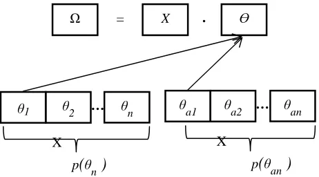
Ɵ and unknown parameters X becomes Ω denotes the universal, Ω=X. Ɵ [5] thus it is important to obtain as many information about the parameters as possible to derive informative results.

Fig. 1 Reduced parameters explained in diagram

As illustrated in Fig. 1 above, conceptually, these are the building block of a universal set Ω which is the outcomes of all possible parameters and the unknown parameters. Given

Ɵ is the space of all possible parameter values θ where θϵƟ. In the diagram, there are two sets of parameters θn and θan. These sets are the element of the parameter space Ɵ. If let say a method is used to reduce or discard each of the parameters set, it will limit the parameter information which could be used to drawn further conclusions or the inability to predict unknown (zero days) attacks. This problem could be solved through prior information.

Rahbarinia, B et al. [6] used pruning rules, for instance, a query rule of ≤ 5 domains, queries ≥ 99.99 percentile, population, query ≥ 1/3 θm meanwhile hereby Zaman, M et al. [7] applied whenever there is i, such that ti≤ t & ti+1 > t and the i is the single parameter θ of the extraction feature of http

which both approaches are limiting the adequate feature information. Edem and Feizollah [8, 9] used the K-mean as the method to reduced noise in feature information as for instance suppose there are two instances of M and N attributed to the coordinated of two parameters of Xij and Yij in an initial centroid value of C1 and C2. The distance is calculated using Euclidean distance, D as below

D = √i=1∑n j=1∑n || xi – xj ||2 + || yi – yj ||2

The process is repeated and Xij and Yij will be grouped again into similar groups based on the new minimum distance to the centroid. This clustering technique tends to ignore the instances that are not the entity of any of the formed clusters thus reduce the parameter, θ information.

Studies from Zaman, Edem and Feizollah [7]-[9] also reveal that previous methods and current behavioural research are highly dependent on instances or sign to feed into the feature selection process. Meanwhile, Villalba and O'kane [10], [11] used n-gram of the given n size of instructions p=I1, I2…In. and, from a N=2 program structure that composed of two opcodes of one or more operands, the operands are then discarded left only the set of opcodes of o:

p=o1, o 2… on. This discarded step will reduce the parameters.

2) Lack of Priori, p(θ): Prior distribution p(θ) describes our belief that θ represents the true population characteristics [5]. As shown in Fig. 2, For instance, research in Wen, S et al. [12] applied state transition which usually depends only on the current state to determine the outcome of the next state and does not take into consideration the outcome of the previous state [13].

Fig. 2 Lack of priori explained in diagram

This is not the case with intrusion and malware detection, whereby any of the previous states or transactions is taken into account. In state transition, Markovian chains, for example, every new stage or the outcome at any stage is called current state. For example, give the following transition:

Pij = P(Xt+1 = j | Xt = i)

= P(X1=j | X0 = i) (2)

The transition shows above only depends only on going one step ahead. It is always Xt = i = 0 and Xt+1 = j = 1, where the state will go from 0 to 1. This will not describe the characteristic of prior knowledge of any event. The limited

priori leads to limited conclusion to be drawn.

Ahmad, Xue and Arora [14]-[16] used ratio, percentage, frequency, average distribution to represent the collection of information of the main features in data collection without determining inferential or in-depth analysis thus lack of prior knowledge, p(θ_{) [17]. In the future, this ratio could be}

applied with additional traffic ratio between application layer protocols with further refinement and representation through Poisson distribution model to enable the generalisation of traffic behaviours throughout the research domain [14].

Xue, et al. [15] assumed the suspicious connection denoted by SP to be larger and of longer duration, which led to the conclusion that whenever a connection packet is more than or equal to ten, n≥10, and the duration exceeds 10 minutes, that connection is considered malicious. This could be true in some instances; however, detailed experimental data should be provided to support such an argument. Prior information is formed using probabilities.

Another example of is the study of Wen, S et al. [12], who assumed that the state of neighbouring nodes is independent and that neighbouring nodes are in the same broadcast domain, although in the real production network

X

= . Ɵ

Ω

θ1 θ2 … θn θa1 θa2 … θan

p

(

)

X

p

(

)

X

X

= . Ɵ

Ω

θ1 θ2 … θn θa1 θa2 … θan

This set is discarded/reduced X

(1)

they are not necessarily in the same collision domain. This assumption shows it lack of priori information.

In a volatile or in a critical infrastructure network environment such as in energy industry, the lack or prior information could cause catastrophic false alarm as happened in the history of Iranian nuclear plant and in Saudi Aramco oil and gas plant.

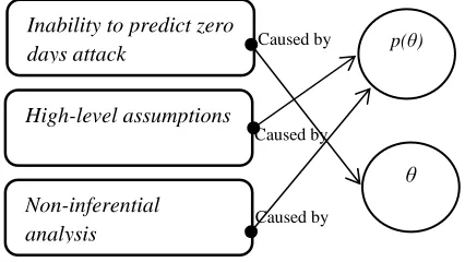
3)Liaison between Issues and Common Criteria: Fig. 3

shows the logical relationship between highlighted issues and the common criteria of the scientific hitches mentioned in subsection A and B. Reduced parameter has been identified causes the inability to predict zero-day attacks mainly because answers of the uncertainty of any distributions or data observations are obtained from how much finite amount of information contained within the data at hand [18]. Parameters θ is a numerical characteristic of a given population or space Ɵ of which often signifies as θϵƟ [4]. This is the building block of the whole universal set Ω, thus obtaining the maximum amount of parameter information is a paramount task for which failure will lead to false alarm and incapability of interpreting future attacks.

Fig. 3 Logical relationship between issues and common criteria

Meanwhile, lack of priori information causes the high-level assumptions and non-inferential analysis. Prior distribution p(θ) describes the preceding scientific belief system that θ represents the true population characteristics [5] and this gives some sort of probability function which could establish the randomness or uncertainty associated with the parameter θ which in turn determine not necessarily the total outcome but also the consequences of the experiment [18]. This could be done by determining the probability function of the parameter at certain values. By contrast, high-level assumptions and non-inferential analysis will never go through such discipline because of the descriptive nature of its analysis where it just represents the collection of information of the main features in data collection without determining inferential or in-depth analysis [17].

Before going any further, some introduction of the background studies of this research is explained here. This paper is the continuation of a few published papers on behavioural analysis which is focusing more on network level analysis. Paper Yusof et al [37] discusses an overview of functionality of malware analysis studies of system and network level from various literature in terms of technical aspects of signature and behavioural based analysis methods which includes Support Vector Machine, Poisson,

Rule-based, Set-Function, Longest Common Sequence, K-Mean Clustering, Relationship Functions and open source which generally categorised as machine learning, statistical and tool based analysis method. Feature selection and evaluation technique in host and network level are also summarized in this paper. Overall in this paper, the epistemological aspect of this research domain is underlined and introduced to the research community with the formation of general malware analysis research framework and a few useful tables that tabulate information with regards to methods previously used in system and network level malware analysis, tabulation of feature selection and evaluation techniques. This paper established the trending area in this research domain which is the behavioural based method which could drive a future researcher to look into this area of studies.

Paper Yusof, M. H. M et al [1] meanwhile further details out the nomenclature of behavioural analysis methods specifically in the area of computer networks. As a continuation of paper [37], it is further confirmed that signature-based analysis that is done statically is no longer sufficient to solve malicious attacks problem, therefore, a behavioural or anomalous analysis will provide a more dynamic approach for the solution. This paper has critically and intensively reviewed more literature especially in the area of behavioural malware analysis studies in the computer networks. It reveals a few shortcomings of previous analysis methods and established a discussion on why Bayesian Network is preferably the best method to cope with the stated problems.

In parallel to that, this paper is designed to introduce the readers to some of the important interdisciplinary topics surround Bayesian Network method more specifically in the area of Clinical Expert Systems, Artificial Intelligence, and Pattern Recognition.

Since the malware analysis in computer networks, in general, are less studied due to the lack of leveraging behaviour of the malware attack in the network environment as mentioned by Nari et al. [38], this paper realised that behavioural analysis research in network level is still a new domain which applies approaches that might have simple knowledge based or statistical approach used to address the scientific hitches, due to that this paper discussed some sophisticated statistical approach that suits in complexes and volatile environment and proven across different disciplines.

B. Related Method

A few methods have been introduced to resolve problems of the shared characteristics of the common criteria from the previous discussion. The solution is basically coming from the current trends in malware analysis method which has been identified as in the class of probability theorem, fuzzy, statistical analysis and clustering [1]. The solutions are rule-based, correlation statistics and state-transition of Markov Chain.

1)Method Overcomes Reduced Parameters θ: One of the

well-known methods for knowledge manipulation and knowledge representation was a rule-based system which has been applied by Zaman and Petel [7], [19] in the form of R1: if θ1 then θ2 where the θ2 statement of consequence can be determined with level of certainty whenever θ1 statement of condition is observed. Let another rule conditions that R2:

θ

p(θ)

Inability to predict zero days attack

High-level assumptions

Non-inferential analysis

Caused by

Caused by Caused by

if θ2 then θ3 where θ3 statement represents the forward chaining factor which involves the rules of R1 and R2 immediately after x1 is established in the chain.

Note that such rules are unbalanced or asymmetric in the sense that the statement of condition and the statement of consequence are not interchangeable (switchable), such that by observing the statement of consequence does not allow us to conclude the statement of the condition [20]. Say, some event m is known to cause the effect in event n and the relationship of both events are known to be deterministic. Hence, the causal relationship between m and n can be formulated as a rule such that “if m then n” rather than “if n then m”.

Rule-based system ignores some mechanisms or causal parameter of "causal direction" which makes this method is assured only up to certain level of precision. For instance, in medical expert systems scenario consider the causal chain of smoking causes bronchitis causes dyspnoea which is denoted by the following concatenation rules as introduced in [20] R3: if smoking then bronchitis and R4: if bronchitis then dyspnoea. Bronchitis is a respiratory infection which is the main airways of the lungs (bronchi) is inflamed and becomes irritated whilst dyspnoea is a medical term for shortness of breath a symptom of bronchitis [21]. Now, let assume that the R4 is formulated as R4 rule which states R’4: if dyspnoea then bronchitis. This statement would make smoking and dyspnoea become contending conditions for bronchitis which consequently would not be able to determine the condition of the patient's breathing patterns. Obviously, the rule based is inappropriate for representing the nature of causal relations amongst events [20] which in turn Bayesian consider every possible rule in the form of

priori and posteriori information to represent the causal

relations.

K-means by Edem and Feizollah [8], [9] then clusters n (the parameters) into K clusters around centroid C, where C= {C1,C2…Ck} given S ={ S1,S2…Sk}, number of partitions. The process of iteration to get new centroid is used to overcome the reduction of parameters; however, this iteration process is based on the ratio between two points. This will further distance the plausible parameter information as at the first place is has been reduced then the iteration makes the plausible information distance even further which finally will draw wrong information.

2)Method Overcomes Lack of Priori p(θ): Correlation

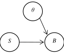
statistics methods as in relational function and average distribution have been closely introduced by Arora, Ahmad, Wen and Xue [12], [14]-[16]. Correlation is a statistical association between two events which often infers or implies causal even if there is not a direct connection relation between the two parameters events. A correlation may signify the occurrence of hidden parameters which are common causes of the observed events, thus makes them statistically associated. Take for instance in Fig. 4 that illustrates the example below of whether smoking denoted by S causes bronchitis denoted by B or whether there exist additional veiled parameters denoted by θ that cause both events which have been introduced by [5].

Fig. 4 Correlation between smoking, S and bronchitis, B and the hidden parameters θ

In a randomized experiment, it is a practice that whenever there is a possibility of unknown hidden parameters, it is necessary to separate the "cause" in order to conclude that there exists a causal relationship which is achieved by a controlled or randomized experiment. For randomized experiment, each level of treatment groups is chosen randomly.

Fig. 5 Correlation between smoking, S parameters θ and bronchitis, B in a controlled experiment

Meanwhile, like in the case of Fig. 5, group of smokers and non-smokers are assigned randomly to carry out "controlled experiment" which consequently leads to the removal of a relationship between hidden parameter θ and smoking S. This is to ensure only the causal connection of interest is observed. This seems to only satisfy the conclusiveness of the association, correlation or relationship between variables which is due to the causal link.

Without the controlled experiment, the results might be unsatisfactory. Thus it is more likely to discover the knowledge of causal relations rather than simply statistical associations that give some sense of genuine understanding, thus in such case, Bayesian networks provide a straightforward expression between variables [5].

In the extension of Wen, S et al. [12]’s state transition of Markov chains a stochastic technique whereby amongst others, the properties are state i and j communicate each is accessible from the other, and once it is in the state i, there is a positive probability that it will never return to state i and if the state is called an absorbing state if the probability of the state is absolute 1, say for instance Pii = 1. Markov chain depends solely on the present state, not the prior or preceding states.

For each Sij, i represents the starting location and j represents the ending location for that move, where the row is the beginning location and the column is the ending location after one move. Each element in the matrix has the probability between 0 and 1, inclusive. The elements of each row of transition have the total probability size of 1 and the

S

θ

B S

θ

B S

θ

B

matrix must be "squared" because it has row and column for each state. As previously stated, stochastic Markovian can usually be determined only by the current condition of the state in order to determine the outcome of the next state; it does not take into account the outcome of any of the previous states [11] and Bayesian network overcomes this limitation by taking consider of prior information through probabilistic inferential.

3)Limitation of Previous Methods: This section

summarizes limitation of previous methods. Rules based are unbalanced or asymmetric in the sense that the statement of condition and the statement of consequence are not interchangeable (switchable), such that by observing the statement of consequence does not allow us to conclude the statement of condition [23], whereby the rule ignores some mechanisms or causal parameter of “causal direction” which makes this method is assured only up to certain level of precision and obviously, the rule based is inappropriate for representing the nature of causal relations amongst events.

K-means iteration process, on the other hand, is based on the ratio between two points. This will further distance the plausible parameter information as at the first place is has been reduced then the iteration makes the plausible information distance even further which finally will draw wrong information. Correlation statistics method seems to only satisfy the conclusiveness of the association, correlation or relationship between variables which is due to the causal link, thus it is more likely to discover the knowledge of causal relations rather than simply statistical associations that give some sense of genuine understanding [18].

Finally, stochastic Markovian can usually be determined only by the current condition of the state in order to determine the outcome of the next state; it does not take into account the outcome of any of the previous states [13].

C. Bayesian Method Solutions

Having realized that rule-based, k-means, correlation and state-transition methods have limitations as a method of reasoning and knowledge representation, researchers switched their devotion towards a more sophisticated probabilistic interpretation of the certainty leading them towards the definition of Bayesian network approach [22].

Bayes's theorem had been pioneered by Tomas Bayes and published in a Posthumous Publication in 1763 which since then had been widely accepted as an uncontroversial result in probability theory [24]. This approach deals with decision-making process under uncertainty conditions or scenarios [25] which in summary it combines the past distribution (prior beliefs) with the available observed datasets to form the posterior distribution.

Bayesian is an inferencing tool that uses past observations (prior belief) to predict the future. Bayesian decision-making process provides an optimum result in classification problem when the prior or past probabilistic history is known which can further derive the estimation or expectation functions [24].

Bayesian Networks is also probabilistic causal networks also known as Belief Networks are the Artificial Intelligence framework for uncertainty supervision which is contrary to

deterministic approach to understand phenomena [26]. Although it was published in 1763 the techniques apply in health management and medicine decision-support systems are quite recent [24] and widely applied in clinical support decision [26]. Bayesian method offers instinctive, meaningful, professional and rational inferential analysis which gives the capability to solve complex situations given the priori distribution in addition to the dataset, thus making decisions easier to clarify and explain [25].

Previous Bayesian Quadratic and Bayesian Linear and models can mislead to false inadequate results due to the great size of parameters that have to be estimated from the dataset thus Naïve Bayes is capable a this issue [24]. Because of the intuitive ability to model uncertainty and complex chronological relationships amongst variables, Bayesian network is successfully applied in several research areas and domains [9,16] and the contribution of this paper is to tailor this general approach to generate new Bayesian Network detection technique to be applied at the Network-level environment [16].

1)Bayesian Method in Clinical Expert Systems: Expert

systems development for clinical diagnosis has received a growing interest in the literature for the past few years [27]. Recent development of the expert systems particularly uses Bayesian is used in planning cardiac surgery for transfusion requirements [28].

Naranjo, L et al. [27] built a Clinical Expert System for the detection of PD using the Bayesian approach due to the traditional diagnosis which involves manual history taking is not definitive diagnostic test. Sometimes the procedure leads to misdiagnosis or even worst undiagnostic, thus there are great necessities to develop scientific systems which can help medical procedures especially in the neurological units. This research involved 80 subjects and 40 of them were healthy and another 40 infected by PD. The mean (± standard deviation) of age for the control and infected group was 66.38 ± 8.38 and 69.5±7.82 respectively. Features selected were from 44 different acoustic sounds from five families of noise, amplitude, pitch, nonlinear and spectral.

Naranjo, L et al. [27] introduced n random variables

Y1…Yn which Yi are observed is in Bernoulli distribution. The probability of success is P(Yi = 1) = pi , i=1…n. The probability of pi are connected to two sets of covariates xi and zi , where xi = (xi1 … xik)

t

is a K x J matrix which is covariate K measured with J replicates, and zi = (zi1…ziH )t is a H vector of a set of H covariates which are precisely identified. Then, suppose that xij = (xi1j… xiKj) is the jth replication of the unknown covariates vector wi = (wi1…wiK) and assume their relationship is linear. This way xij are the substitutes or surrogates of wi. The following model relates

xij and zi.

Yi ~ Bernoulli (pi), Ψ-1 _(p

i) = wtiβx + zti βz (3)

xij = wi + εij (4)

εij ~ NormalK (0, G), indicates error vector

where β = (βtx , βtz)t is a (K + H) vector of unknown

parameters, then Ψ-1 (.) is a known nonnegative function or

link function ranges between 0 and 1, and G is a K x K matrix of covariances and variances. εij error vector is independent of wi. Typically, Ψ(.) is the CDF (cumulative distribution function) or normal distribution. To define prior distribution is to assumed normal distribution of the regression parameters, β ~ NormalK+H (b,B) and it is assumed prior distributions covariance and variance parameters G ~ InvWishartK (V,v), where b , B , v and V are fixed and wi ~ NormalK (μ,Σ) where μ,Σ are also fixed. Likelihood function is

Ɩ (β, G | y, x, z, w) = f (y | z, w, β) f(x | w, G) f(w), (5)

then the posterior density is

π (β, G | y, x, z, w) ∞Ɩ (β, G | y, x, z, w) π (β)π(G) (6)

where this approach makes use of the relationship between covariates and prior distributions to achieve posterior distributions. Fig. 6 below clearly shows the Bayesian model used in this research. Spotted easily several conditional probabilities networked together to the priori to derive posteriori distribution. Results are validated uses stratified cross-validation, but before results from precision (TP/TP+TP), recall rate (TP/TP+FN) and specificity (TN/TN+FP) are obtained.

Fig. 6 A Bayesian model to determine Parkinson’s disease

Next, Miasnikof, et al. [29] classified verbal autopsies (VA) which are largely adapted in low-income countries uses Naïve Bayes classifiers. This is due to no reasonable standard to validate the practice which had become the cause of home death, thus the studies pursue to measure results from Naïve Bayes classifier against existing standard procedures which is using physician classification. The dataset used is from Million Death Study, Matlab Bangladesh, and Agincourt South Africa. Sample sizes were 12,255 which contained deaths at ages 1to 59 months, 15 to 64 years, 20 to 64 years and 28 days to 11 years. For every autopsy (VA), a probability (priori) will be assigned to each autopsy label, which is a specific feature in the form of symptom or sign, in accordance with their conditional probabilities. Only label with the maximum probability will be assigned to each label records. Suppose Cj* is the cause of death, given a set of n records of signs and symptoms which are denoted by F1…Fn.

Cj* = arg max.j {Pr(Cj | F1…Fn)} (7)

Since the labels or features are chosen with the maximum probability, each feature Fn in the above equation is either 1 if the symptom is reported in VA and 0 if otherwise, and for simplification, the notation will be Pr (Fi = 1 or otherwise). Thus the proportional relationship of the above equation will be

this is the posteriori

Then is to apply the Bayesian assumption of the maximum probability to derive the following equation

Pr(Cj | F1….Fn) ∞ Pr(Cj) . π ni=1 [ ]i Pr(Fi | Cj) + (1-]i) (1- Pr(Fi | Cj)) (9)

where,

]i = { 1 if feature i is reported

0 otherwise

Pr(Cj) = | Cj | / N (10)

where N is the size of features (total number of features)

(11)

Priori distribution in this equation is just a proportion of sample cases |Cj|, against the total number of features. Whilst | Fi⋂ Cj | is denoted as the total number of causes of death that showed feature Fi. The results will be evaluated against testing splits of the datasets to measure sensitivity or True Positive Rate (TPR) and specificity or False Positive Rate (FPR).

Meanwhile, Fuster-Parra, P et al. [26] applied Bayesian Network to determine the relationship between pertinent epidemiological signs of heart. For instance, given a set random variables X= (X1…Xn). The prior distribution as a product of several conditional distributions is

Where Pa(Xi G

) denotes the parent prior distribution which uniquely signifies the multivariate formulation in Bayesian Network which is also known as Bayesian Network chain rules. To enable inferential analysis, it is important to understand the flow of influence when any new information is introduced in Bayesian Network. For instance, let two variables X and Y which are separated by Z at several possible paths. X Z Y or X_Z_Y which is known as a serial connection, X_Z Y as diverging connection and Z is initiated and finally, X ZY which is known as converging connection where Z hasn’t receive evidence. In this research, Bayesian was validated through 10-fold cross-validation uses log-likelihood loss function.

In medicine, Bayesian Network could characterize the conditional probabilistic value between symptoms and the diseases. Barbini, E et al. [24] shows a good illustration of

p[i]

βx βz

Z[i]

Z[i]

Y[i]

(8)

Bayesian Network applied in Clinical Expert Systems, where Bayesian Network is presented in a directed acyclic graph which has nodes and arcs. A node represents a random variable and an arc represents the conditional probability between nodes or variables.

Fig. 7 below illustrates their Bayesian Network model. For instance, between node A and node C, there is an arc representing the conditional probabilistic relationships. It also indicates that A has influence on C or A is the parent of node C as mentioned by [26]. There exist nodes, C and D, which are not connected to each other or lack of arc between them; this is to indicate that their existences are mutually exclusive and conditionally independence of each other. Nodes C and D which have parents' nodes are regarded by their conditional probabilities characteristic which are table systematically. Meanwhile, parents' nodes which in this case node A and B are regarded as priori or prior probability. Consequently, P(A) is denoted as the probability of any event A and xA’B denotes the probability of any event C gave event B but not event A. On the occasion of all possible events of Bayesian Network have been defined, prior distribution of the parents' nodes and conditional probabilistic value of the inheritance should be specified.

Fig. 7 A Bayesian model with two parent’s nodes and two variables

As a conclusion, Bayesian Network is about several experts' structures which are combined or connected together to form a dependencies domain.

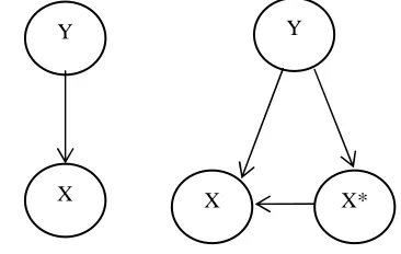
2)Bayesian Method in Pattern Recognition: Wang, et al.

[30] proposed two and three nodes Bayesian Network model to recognise spatial age-related expression labels as shown in Fig. 8. Bayesian Network in this work represents a joint probability distribution amongst a set of features. As in Fig. 8, each node represents the features points and the arc or the link between nodes represents their conditional distribution probability which shows the probabilistic relationships between features points. Diverse Bayesian Network expressions were constructed to condition various spatial facial patterns amongst different expression and age.

This work was preluded with several activities such as forming two statistical hypothesis tests to scrutinise the

effect of age on spatial patterns of facial expression using ANOVA. After both hypothetical tests were conformed the two Bayesian Network model were applied. Bayesian Network discovers relationships amongst facial landmark points.

Fig. 8 Two nodes and three nodes Bayesian Network model

Throughout training a probabilistic model of P(x,x*,y) is used, whereby the training set of (xi,x*i,yi) given i=1…l and

xi are features data in geometric distribution, x*i is the age data and yi is the label of expression. The label has priori of P(y = k) (k = 1, 2,…m), where m is the size of expressions and the conditional probability of P(x|y = k) and P(x|y = k,

x*i) are assessed within Maximum Likelihood method. It is understood that (xi,x*i,yi) is the training set where i=1…l and l is the size of training samples. The posterior probability of

P(y = k|x) is calculated during this data training exercise and

follow the following expression:

Where conditional probability of P (x*|y=k) can be characterised as Gaussian or Normal distribution P (x | x*, y = k) ~ Normal (x | μi

(k) , Σi

(k)

) where i=1,2….n and n is the size of the age groups for each x* and x* has n states. In this work, it is obvious that every x* is converted or encoded into the conditional probability of P (y|x).

Meanwhile for the probability of P (x|y) of the two nodes Bayesian Network model as in Fig. 3 also often conforms to a single Normal Distribution, however, the three nodes model with discrete x* can improve the conditional distribution of P (x|y). This research further constructed different Bayesian Network under different condition of expression and age. For instance, age group data is also regarded as controlled information, hence m x n Bayesian Network model of Gc with c = 1…m x n are constructed during the training period. Then, for every Gc parameter that is learned from the training set xc = (xci)i=1lc where xci = (fci1,

fci2… fciP) and p is size of the features. This model is to learn the highest network score or the best xc.

Suppose priori of Gc with c = 1…m x n is uniform in distribution, thus during training we get P(Gc|x) ∞ P(x|Gc). Subsequently for every continuous node the probability are normal or Gaussian where the parameter is defined as fj ~ Normal (bj + Wj

T

Pa(fj), δj 2

), where j = 1…p, Pa(fj) is the

Y Y

X _{X X*}

C

A B

D

P(B) P(A)

A B P(C|A,B) True True

x

x

x

x

B P(D|B) True

y

y

(13)

parent’s state of fj, Wj signifies regression coefficients, bj denotes regression intercept and δj2 shows the variance. Score function below shows the search strategy to learn Gc.

where θc is the parameter given Gc

The following Maximum Likelihood method is used to estimate the parameter of given Gc mentioned above, where

θc signifies parameter set of cth Bayesian model.

θc = argmax log P(x | θc) (15) Then the following expression is to signify the testing set into maximum likelihood method

c* = arg max c ϵ [1, m x n] P (ET | Gc)

Complexity (Gc) (16)

Where ET denotes sample features, Gc signifies the cth Bayesian model where the c ranges from 1 to m x n, P (ET |

Gc) denotes the probability of the sample features the cth model, and complexity signifies the complexity of Gc this is due to diverse differences amongst spatial structures, thus the probability of P (ET | Gc) will be divided by complexity to seek the balance. Finally, the method is validated through ten-fold cross validation.

Meanwhile, Mihoub et al. [31] model face-to-face multimodal behavioural of co-verbal communication uses dynamic Bayesian Network method where it is a classical basic sophisticated multimodal bidirectional co-verbal communication which allows the partners to recurrently perceive, convey co-verbal movements such as body, hand and arm gestures and head movement.

Thirty games were constructed in which the trainer acted together with 3 different subjects or partners. The game objective is to place 10 cubes at random arrangement for which each game has a mean duration of 1 minute and 20 seconds. This interaction were modelled with 5 variables which are the IU denotes the interaction units which have another 6 different IUs of get, seek, point, indicate, verify and validate, the MP signifies manipulator gestures which have 5 values of rest, grasp, manipulate, end and none, the SP for the instructor speech with 5 values of cube, preposition, reference cube, else and none, the GT denotes the region of interest pointed out by the trainer's index finger which consists of 5 values of rest, target location, cube and reference cube and final variable is FX denotes gaze fixations of the trainer which have another 8 areas. FX and MP were annotated uses Pertech video. SP is transcribed uses speech recognition software. GT was annotated uses Qualys signals and finally IU is manually annotated on every gaze event. Elan software is used to manage multimodal scores.

Bayesian behavioural statistical model of Murphy [32] was used. Bayesian is considered as a probabilistic graphical model that provides conditional relationship representation of several stochastic conditions [33]. In Bayesian Network

an acyclic directed graphs of nodes and edges are represented uses conditional probabilities. For instance, an edge connecting between parent’s node X to child’s node Y signifies that node X has influence over node Y. Sometimes this relationship is learned from the data as in this research whereby the intra-slice structure is derived from K2 and REVEAL algorithm, whereby for K2 algorithm each node initially has no parents, thus this algorithm gradually, adds a parent. The order adopted was IU, MP, SP, GT and FX which shows the interaction unit stays in the first level and the sensory motor at the lower level as shown in Fig. 9.

Fig. 9 The learned structure of Bayesian Network

Interesting properties have been discovered from this learned structure. The interaction unit, IU, stimulates both perception and action units. The MP impacts the SP, GT and FX. The SP or speech activity influences verbal or action behaviours of GT and FX. In essence, each random variable is influenced by its history or learned parents. For validation, this model is compared with the state-of-the-art baseline model which is Hidden Markov Model (HMM).

3)Bayesian Method in Malware Analysis: Kao, et al. [34]

proposed a Bayesian of nonparametric approach to determine a malicious or benign at system level program under several first-order assumptions which have been modeled uses Dirichlet process mixture model. Let N represents the size of sample programs s, where s=1…N. Dynamic trace of sth program is signified by {Ys1…YsNs} where Ystϵ {1…M} is the tth element during instruction call, Ns is the size of dynamic trace and M is the size of classes of instructions which implies that any similar instruction will be classed into similar group. To model first-order Markov structure it is enough to model distribution of first instruction Ys1 and M x M transition matrix Zs

SP IU

FX MP

GT * Interaction

unit

Perception units

Action units (14)

Zsrc = t=2ΣNs I (Yst-1= r, Yst= c), where (r,c) is the element of {1…M}

Both the first instruction and transition matrix distribution are permitted to fluctuate by programs. The first instruction of program s has probability distribution function of P(Ys1 = j)=qsj with j=1ΣM qsj =1. The subsequent or second instructions, t=2…Ns are modelled as P(Yst = c| Yst-1= r)=Psrc with c=1ΣM Psrc =1 for all r. Ps signifies the matrix of M x M with (r,c). Usually, Ns is very large that makes the first instruction Ys1, is less information about the dynamic trace characteristic, thus it can be disregarded. In this case, matrix transition Zs is sufficient for the dynamic trace statistic information, which then derives the following likelihood function for one single program of s,

f(Zs | Ps ) = r=1ΠM , c=1ΠM PsrcZsrc

The probability of the transition matrix Ps for a single program s is assumed Ps ~ F for any s, and where F probability distribution of matrices across malicious programs. The prior information of F is placed in non-parametric form to increase flexibility whereby F is assumed by Dirichlet process of Bayesian model

Ps ~ F

F ~ DP (a, Fb) (18)

Where a>0 is concentration variable and Fb is the base distribution of the prior Dirichlet process. Large a pushes F

priori closer to Fb, in this research Fb is distributed by matrix Dirichlet (MD), Fb = MD (yP). Meanwhile, Dirichlet priori can be denoted as density mixture of

f(Ps| w, λ) = k=1Σ∞ wk . δ(Ps | λk) (19) where λ = {λk : k=1…∞}, wk = {wk : k=1…∞} and wk > 0 fulfil k=1Σ∞wk=1 , δ signifies Dirac Delta density at point mass Ps = λk and λk ~ Fb .

However, this Dirichlet process has a discrete distribution which gives the transition probability is not appropriate, because the two probabilistic transitions of two executables could be identical and this is unrealistic. Therefore, the priori should be considered as in the next form of equation

Ps | θs, o ~ F = MD (o θs)

θs | G ~ G

G ~ DP (a, Fb) (20)

where the parameter o>0 controls the variance of Ps distribution. By having this equation, probability of two identical transition matrices will be equal to 0. On the full model of Bayesian classification another variable is introduced, ξs where

ξs=1 if program s is malicious 0 if program s is benign

Where P(ξs=1)=ψ is the priori of being malicious. The following illustrates Bayesian model on a single program s

f(Zs | ξs = i , Oi ) = k=1Σki wik . fMMP (Zs | λik, oi), i = 0,1

λik ~ MD (yi Pi) (21) ξs ~ Bern (ψ)

where O0 = { λ0, y0, o0, w0, K0} and O1={ λ1 y1 o1 w1 K1}are all the pool of parameters beneath the malicious and benign models that allow different malicious and benign programs that are with different mixture densities and base distributions. Finally, the validation is against existing support vector machine (SVM) and elastic net logistic (ENL) regression method. In the case of generating a parametric form of the conditional probability functions is not possible Non-parametric approach is used, however, this approach is complex [1] and will not be suggested as a future research. However, the essence of establishing prior, conditional and posterior distribution as in the Bayesian theorem will be applied in the proposed method.

On the other hand, Weaver [35] modeled bot net scanning behaviour in a large network environment as she claimed the sandbox environments seldom emulate real user experience. Furthermore, NAT and DHCP configuration have made the IP in ISP level doesn’t map one-to-one and the real perpetrator will not be revealed. However, from the point of view of experienced network engineer or administrator, it is true that the NAT will translate outbound and inbound traffic, but each organisation will be assigned unique IP address to make them online in the large network, however it is the work of local administrator to stream down or deep inspect the flow to identify the source and destination IP within the local area network.

The monitored network was from large private network from the period approximately 2 months window from the month of March 5th until the month of April 24th. The network flows were collected uses flow analysis toolset of SiLK or System for Internet-Level Knowledge which is available at tools.netsa.cert.org/silk and the features monitored were from the source IP address, timestamp and source port. Accumulated around 33.6 million total unique IP addresses were monitored disbursed across 1.1 million /27 IP blocks. Behaviours show fluctuated events of periodic inactivity which indicates consistent machine shutting down activities and several spikes which indicate starting of new activities. The model was from the single machine connection rates of several user activities such as web surfing or switching the machine off or on. This is the alternative behavioural model of counting infected machines from the layered network blocks or IP addresses. λt, denotes the Poisson mean of the number of connection requests, yt in,

t hour (yt ~ Poisson (λt)), where λt = q (1+ ak (ɷ-1)) such that

q denotes the baseline rate, a denotes the decay rate, k

denotes a spike after an active hour and ɷ denotes a spike multiplier. A steady rate is denoted by q (baseline rate) and occurs when the host is idle. The state of the user’s machine or system is denoted by η, represented by three states of possibilities which are “o=off, s=spike, d=decay”. A host is said to be in the “off” state when there is no connection request, yt = 0 with probability=1.0. When a host is active, three conditions are applicable; a geometric decay at rate a, a multiplier spike at ɷ >1 and a baseline at rate q.

A set of transition probabilities between spike and decay of the user’s state η to η+1 hour-to-hour is modelled uses (17)

geometric distribution with rates of yt and yd, meanwhile transitions between non-equal user’s state, off-to-spike, spike-to-decay and off-to-decay is modelled uses sine wave with maximum height of p and scaling amplitude of v within 24-hour cycle and t*, an hour a day will be between 0 to 23. Thus the transitioning state between s2 to s1 is denoted by

Ps2 | s1 (ps1, vs1, t*) = (ps1/ (vs1+2) ) [sin (2π t* / 24) + vs1 + 1] (21)

Next, is to build probability model of machine and user’s activity uses Gibbs sampling a method of Markov Chain Monte Carlo in order to explore the posterior distributions [17] by considering several relevant prior information. Suppose η is the machine state at time t: ηtϵ {o, s, d} and η = {η0… ηT} and y={y0…yT} as the observed vectors, subsequently let ψ = {p{ o, s, d }, v{ o, s, d }, y{ o, s, d }, λoff} be the probability of user’s transitional activities and θ=(q,w,a) be the machine-level parameters. The likelihood would be the joint of all distribution given earlier, Ɩ (ψ, θ, η;y).

Gibbs sampling explores posteriori by initiating value for the entire parameters and iteratively straws new values for a subsequent subset based on the conditional probability of those parameters and Markov chain derived from this chains of iteration is the joint posteriori for the entire parameters [8]. For instance, let φϵ (ψ, θ, η) with priori of π (φ) and let {ψ, θ, η}| φ be the observed vectors for the entire parameters

except for φ. The complete general conditional probability distribution is

π (φ | {ψ, θ, η}| φ, y ) = π (φ) Ɩ (φ, { ψ, θ, η }| φ; y)

ʃφπ (φ) Ɩ (φ, {ψ, θ, η}| φ; y) (22)

Boukhtouta, et al. [36] compared several machine learning techniques such as J48, Naïve Bayesian and Support Vector Machine to detect malicious activity at the network level as the state-of-the-art Intrusion Detection Systems (IDS) uses signature-based techniques to filter bad traffic is insufficient. The non-malicious traffic was obtained from Defence Advanced Research Project Agency (DARPA) trusted source. However, the research is a software suite-based approach which makes it difficult to evaluate the analysis engine.

III.RESULTS AND DISCUSSION

The previous section discusses various application of Bayesian Network in several domains like Clinical Expert Systems, Pattern Recognition and reminiscent of Bayesian work in malware analysis. In essence, Bayesian network is a directed acyclic probabilistic model that represents a set of random variables and their conditional probabilistic relationships.

There are a few properties encompasses Bayesian Network method. Statistically, a Bayesian Network model has four properties which are 1) prior probability or priori, 2) the likelihood or the conditional probability, 3) posterior probability or posteriori and finally 4) the relationship of parents’ nodes and its inheritance. For instance, given a prior information of y and parameter θ, the priori would be p(θ) and the conditional probability is p(y | θ) and generated posterior would be

p(θ | y) ∞ p(y | θ). p(θ) (23) Frequently in Bayesian Network, the priori rest on to other parameters φ that are not declared in the conditional probability or the likelihood, thus the prior p(θ) must be substituted by the conditional probability of p(θ | φ). The newly elected parameters φ posteriori would be

p(θ, φ | y) ∞ p(y | θ). p(θ | φ). p(φ) (24)

Based on the literature, studies from Clinical Expert Systems have the full four properties in their expert systems model, whilst domain like pattern recognition and existing malware analysis studies fulfill the first three out of four of Bayesian or Naïve Bayes properties. The four properties discussed here addresses problems in the common criteria.

IV.CONCLUSIONS

This paper discusses the application of Bayesian Network model in various domains such as Clinical Expert Systems, Artificial Intelligence, Pattern Recognition and reveals any potential approach available in the domain of Computer Networks. It is discovered that Bayesian (Naïve Bayes) method has been applied in the malware analysis domain both in network and system-level behavioural analysis. However, this method has several issues in dealing with zero-day attacks which are related to the issue of predicting future attacks pattern. Based on the literature Bayesian Network properties which have been applied in various domains could have the potential to overcome those problems. Thus these properties could be used as guidance for future studies on modeling Behavioural Malware Predictive Analytics at the network level.

ACKNOWLEDGMENT

We would like to thank Faculty of Information Science and Technology, Universiti Kebangsaan Malaysia for supporting this research using research grant code DPP-2014-014.

REFERENCES

[1] M. H. M. Yusof and M. R Mokhtar, “The Nomenclature of Behavioural Malware Analaysis Methods in Computer Networks”. Security and Communication Networks. Id: SCN-16-0424, 2016 [2] D. S. K Rai. “Performance Based Comparative Analysis of AODV,

DSR and DSDV Protocols”. Master Thesis. Computer Science and Engineering Department Thapar University. 2009.

[3] H. D. Trung, W. Benjapolakul, and P. M. Duc, “Performance evaluation and comparison of different ad hoc routing protocols,” Journal of Computer Communications, vol.30, pp. 2478-2496, 2007. [4] P. D Hoff, A First Course in Bayesian Statistical Methods, Seattle

WA, USA: Springer. 2009.

[5] T. Koski, and J. M. Noble, Bayesian Networks, United Kingdom, John Wiley & Sons, Ltd. 2009.

[6] B. Rahbarinia, R. Perdisci, and M. Antonakakis, “Segugio: Efficient Behavior-Based Tracking of Malware-Control Domains in Large ISP Networks”, in 45th Annual IEEE/IFIP International Conference on Dependable Systems and Networks, 2015, pp. 403-414.

[7] M. Zaman, T. Siddiqui, M. R. Amin, and M. S. Hossain, “Malware Detection in Android by Network Traffic Analysis,” Next Generation Mobile Apps, Services and Technologies (NGMAST), pp. 66-71, 2015 [8] E.I. Edem, C. Benzaid, A. Al-Nemrat, and P. Watters, “Analysis of Malware Behaviour: Using Data Mining Clustering Techniques to Support Forensics Investigation”, in Fifth Cybercrime and Trustworthy Computing Conference, 2014, pp. 54-63.

[9] A. Feizollah, N. B. Anuar, R. Salleh, and F. Amalina. “Comparative study of k-means and mini batch k-means clustering algorithms in android malware detection using network traffic analysis”, in International Symposium on Biometrics and Security Technologies (ISBAST), 2014, pp.193 - 197.

[10] L.J.G. Villalba, A. L. S. Orozco, and J. M. Vidal,. “Malware Detection System by Payload Analysis of Network Traffic,” IEEE Latin America Transactions,13(3), 2015.

[11] P. O'Kane, S. Sezer, and K. McLaughlin. “N-gram density based malware detection,” in World Symposium on Computer Applications & Research (WSCAR), 2014, pp. 1-6.

[12] S. Wen, W. Zhou, J. Zhang, Y. Xiang, W. Zhou, W. Jia, and C. C. Zou, “Modeling and Analysis on the Propagation Dynamics of Modern Email Malware”. IEEE Transactions on Dependable and Secure Computing, 11(4), pp. 361 - 374.

[13] J. G. Kemeny, J. L. Snell, A. Knapp, Markov Chains, Pearson Education, Inc. 2003.

[14] M. A. Ahmad and S. Woodhead, “Containment of Fast Scanning Computer Network Worms,” in Proceedings of the 8th International Conference on Internet and Distributed Computing Systems, 2015 vol 9258, pp. 235-247.

[15] L. Xue, and G. Sun, “Design and Implementation of Malware Detection System based on Network Behavior,” Security And Communication Networks, Volume 8 (3), pp. 459-470, Feb. 2015. [16] A. Arora, S. Garg, and S. K. Peddoju, “Malware Detection Using

Network Traffic Analysis in Android Based Mobile Devices,” in Eight International Conference on Next Generation Mobile Apps, Services and Technologies, 2014, p. 66-71.

[17] P. S. Mann, Introductory Statistics, 8th _{Edition. Wiley, ISBN:} 978-1-118-17224-7, 2012.

[18] D. Sorensen, and D. Gianola, Likelihood, Bayesian and MCMC Methods in Quantitative Genetics. New York, USA: Springer, 2002. [19] K. Patel and B. Buddadev, Detection and Mitigation of Android

Malware Through Hybrid Approach, J. H. Abawajy, S. Mukherjea, S. M. Thampi, A. Ruiz-Martinez, Ed., Security in Computing and Communications: Third International Symposium, SSCC 2015, Kochi, India, pp. 455-463.

[20] U. B. Kjaerulff and A. L. Madsen. Bayesian Networks and Influence Diagrams: A Guide to Construction and Analysis. Aalborg, Denmark, Springer, 2008.

[21] (2016) Health and Social Care Information Centre. Bronchitis.

[Online]. Available:

http://www.nhs.uk/conditions/Bronchitis/Pages/Introduction.aspx website 2016

[22] R. E. Neapolitan. Learning Bayesian Networks. Northeastern Illinois University, Chicago, Pearson Prentice Hall, 2004.

[23] H. D. Trung, W. Benjapolakul, and P. M. Duc. “Performance evaluation and comparison of different ad hoc routing protocols”. Journal of Computer Communications, vol. 30, pp. 2478-2496, 2007.

[24] E. Barbini, P. Manzi, and P. Barbini. Bayesian Approach in Medicine and Health Management, A. J. Rodriguez-Morales, Ed., 2013. [25] J. W. Sheppard, and M. A. Kaufman, “A Bayesian approach to

diagnosis and prognosis using built-in test,” IEEE Transactions on Instrumentation and Measurement, vol. 54(3), pp. 1003-1018, 2005 [26] P. Fuster-Parra, P. Tauler, M. Bennasar-Veny, A. Lig˛eza, A. A

L´opez-Gonz´alez, A. Aguil´o. “Bayesian Network Modeling: a Case Study of an Epidemiologic System Analysis of Cardiovascular Risk”. Computer Methods and Programs in Biomedicine, 2015.

[27] L. Naranjo, C. J Perez, Y. Campos-Roca, and J. Martin. “Addressing voice recording replications for Parkinson’s disease detection”, Expert Systems With Applications, May 2016.

[28] G. Cevenini, E. Barbini, M. R. Massai, and P. Barbini, “A naïve Bayes classifier for planning transfusion requirements in heart surgery” Journal of Evaluation in Clinical Practice, vol.19(1), pp 25-29, 2013.

[29] P. Miasnikof, V. Giannakeas, M. Gomes, L. Aleksandrowicz, A. Y. Shestopaloff, D. Alam, S. Tollman, A. Samarikhalaj, P. Jha, “Naive Bayes classifiers for verbal autopsies: comparison to physician-based classification for 21,000 child and adult deaths,” BMC Medicine, vol. 13(1), 2015.

[30] S. F. Wang, S. Wu, Z. Gao, Q. Ji, “Facial expression recognition through modeling age-related spatial patterns,” Multimedia Tools And Applications, vol. 75(7), pp. 3937-3954, 2016.

[31] A. Mihoub, G. Bailly, C, Wolf, F. Elisei, “Graphical models for social behavior modeling in face-to face interaction”, Pattern Recognition Letters, vol. 74, pp. 82-89, 2016.

[32] K. P. Murphy, “Dynamic Bayesian networks: representation, inference and learning”, PhD Thesis, University of California, Berkeley, 2002.

[33] D. Koller, and N. Friedman, Probabilistic Graphical Models: Principles and Techniques, The MIT Press, 2009.

[34] B. Kao, C. Reich, Storlie, and B. Anderson, “Malware Detection Using Nonparametric Bayesian Clustering and Classification Techniques”, Technometrics, vol. 57(4), pp. 535-546, 2015. [35] R. Weaver, “Visualizing and Modelling the Scanning Behavior of the

Conficker Botnet in the Presence of User and Network Activity”. IEEE Transactions on Information Forensics And Security, vol. 10(5), pp. 1039-1051, May 2015.

[36] A. Boukhtouta, N. E. Lakhdari, S. A. Mokhov, and M. Debbabi, “Towards Fingerprinting Malicious Traffic,” Procedia Computer Science, vol. 19, pp. 548-555, 2013.

[37] M. H. M. Yusof, and M. R. Mokhtar, “A Review on Taxonomy of Malware Analysis Studies,” Advanced Science Letters, vol. 22, 2016. [38] S. Nari, A. A Ghorbani, “Automated Malware Classification based on Network Behavior,” in International Conference on Computing, Networking and Communications, Communications and Information Security Symposium, 2013, pp. 642-647.