Volume 6, Number 2, pp. 1–12. http://www.scpe.org c 2005 SWPS
AN APPROACH TO PROVIDING SMALL-WAITING TIME DURING DEBUGGING MESSAGE-PASSING PROGRAMS
NAM THOAI∗ AND JENS VOLKERT†
Abstract. Cyclic debugging, where a program is executed repeatedly, is a popular methodology for tracking down and eliminating bugs. Breakpointing is used in cyclic debugging to stop the execution at arbitrary points and inspect the program’s state. These techniques are well understood for sequential programs but they require additional efforts when applied to parallel programs. For example, record&replay mechanisms are required due to nondeterminism. A problem is the cost associated with restarting the program’s execution every time from the beginning until arriving at the breakpoints. A corresponding solution is offered by combining checkpointing and debugging, which allows restarting an execution at an intermediate state. However, minimizing the replay time is still a challenge. Previous methods either cannot ensure that the replay time has an upper bound or accept the probe effect, where the program’s behavior changes due to the overhead of additional code. Small waiting time is the key that allows to develop debugging tools, in which some degree of interactivity for the user’s investigations is required. This paper introduces the MRT method to limit the waiting time with low logging overhead and the four-phase-replay method to avoid the probe effect. The resulting techniques are able to reduce the waiting time and the costs of cyclic debugging.
Key words. Parallel debugging, checkpointing, message logging, replay time, probe effect
1. Introduction. Debugging is an important part of software engineering. Obviously, a program is only valid if it runs correctly. A popular traditional method in this area is cyclic debugging, where a program is run repeatedly to collect more information about its intermediate states and finally to locate the origin of errors. A related technique often used in cyclic debugging is breakpointing. It allows programmers to stop and examine a program at interesting points during execution.
Parallel architectures and parallel programming have become the key to solve large-scale problems in sci-ence and engineering today. Thus, developing a debugging mechanism for parallel programs is important and necessary. Such a solution should support cyclic debugging with breakpointing in parallel programs. However, in parallel programs, communication and synchronization may introduce nondeterministic behavior. In this case, consecutive runs with the same input data may yield different executions and different results. This effect causes serious problems during debugging, because subsequent executions of a program may not reproduce the original bugs, and cyclic debugging is ad hoc not possible.
To overcome this irreproducibility effect, several record&replay techniques [11, 15, 23] have been proposed. These techniques are based on a two-step approach. The first step is arecord phase, in which data related to nondeterministic events are stored in trace files. Afterwards, these trace data are used as a constraint for the program during subsequentreplay phases to produce equivalent executions.
A major problem of this approach is the waiting time because programs are always re-started from the beginning. Especially with long-running parallel programs, where execution times of days, weeks, or even months are possible, a re-starting point at the beginning is unacceptable. Starting programs from intermediate states can solve this problem. Such a solution is offered byIncremental Replay techniques [31]. They support to start a parallel program at intermediate points and investigate only a part of one process at a time. As an extension, the goal of our approach is to stop at an arbitrary distributed breakpoint and to initiate re-execution of the program in minimum time and with a low overhead.
Requirement to construct adequate recovery lines on multiple processes was previously described in literature on fault tolerance computing as well as debugging [1, 5, 8]. The restriction of these methods is that recovery lines, which are global states that the program can be restarted, are only established at consistent global checkpoints, because inconsistent global states prohibit failure-free execution. Therefore, limiting the rollback distance, which is the distance between the recovery line and the corresponding distributed breakpoint, is impossible. Some additional techniques allow to shorten the rollback distance but the associated overhead may be rather high because many checkpoints are required and a lot of messages must be logged [28]. Both represent serious obstacles during developing debugging tools, which must provide some degree of interactivity for the user’s investigations.
∗Faculty of Information Technology, HCMC University of Technology, 268 Ly Thuong Kiet Street, District 10, Ho Chi Minh
City, Vietnam ([email protected]).
†GUP Linz, Johannes Kepler University Linz, Altenbergerstr. 69, A-4040 Linz, Austria/Europe ([email protected]).
P
1 0
C C
C C C
2
P P
C0,0
1,0
2,0 2,1 1,1
2,2
m1
0,1
C
C1,2
0,2
C
m3 C2,3
2
m
I2,1
C1,3 C0,3 B0
B1
B2
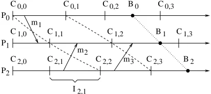
Fig. 2.1.Event graph and checkpoint events.
To solve the above problem, a new replay technique has been developed: theShortcut Replaymethod [29] allows to construct flexible recovery lines and thus the rollback distance is shortened. However, the overhead of message logging is still high. Therefore, the trade-off between the rollback distance and the message-logging overhead should be examined. The Rollback-One-Step method (ROS) [28] is an effort to address this problem by establishing an upper bound of the rollback distance. However, the replay time depends on the number of processes and may be rather long with large-scale, long-running parallel programs (as discussed in Section 5.2). A new method, named MRT (the Minimizing the Replay Time method), is presented in this paper. It ensures the upper bound for the replay time, which is independent of the number of processes. An implementation of MRT and its result demonstrate the efficiency of this approach.
Another important point in debugging is that the observation should not affect the actual behavior of the program. However, the instrumented code and checkpointing activities may substantially affect the behavior of the program. Therefore, the four-phase-replay method is offered as a replay method for MRT with low overhead. This paper is divided into 10 sections. Basic definitions of parallel programs, the event graph and check-pointing are described in Section 2. Definition of distributed breakpoint is introduced in Section 3. Section 4 explains the reason of nondeterministic behavior of parallel programs and provides an overview of record&replay methods to solve the nondeterminism problem. The definition of the rollback/replay distance is also given in Section 4. ROS and its limitations are shown in Section 5. After that, MRT is introduced in Section 6 and its implementation is described in Section 7. The four-phase-replay method to avoid the probe effect is presented in Section 8. A comparison between MRT using the four-phase-replay method and other methods as well as the future work to integrate MRT into the Process Isolation technique are discussed in Section 9. The paper finishes with conclusions in Section 10.
2. System model. The parallel programs considered in this paper are message-passing programs, which include n processesP0, P1, . . . , Pn−1 that exchange data through messages. To model a program’s execution,
the event graph model [11] is utilized. This model describes the interesting operations in all processes and their relations. An event graph is a directed graphG= (E,→), where the non-empty set of eventsE is comprised of the eventsep,i ofGobserved during program execution, withidenoting the sequential order on processPp.
The relations between events are “happened-before” relations [14]. Letep,i→eq,j denote thatep,iis
happened-beforeeq,j and there is an edge from eventep,i to eventeq,j in Gwith the “tail” at eventep,i and the “head”
at eventeq,j.
In our message-passing programs, the event set E contains two kinds of event. The first kind are com-munication events. Only events, which concern sending and delivering of messages, are interesting. They are called send and receive events, respectively. In order to obtain these events for a particular program run, the program’s source code is instrumented and re-execution is initiated. The events (and corresponding data) are stored in trace files.
The second kind of events are checkpointing events, which represent local checkpoints. A local checkpoint is the local state of a process at a particular point in time. The i-th local checkpoint taken by process Pp
is denoted byCp,i. We assume that process Pp takes an initial checkpointCp,0 immediately before execution
begins, and ends with a virtual checkpoint that represents the last state attained before termination. Thei-th checkpoint interval of processPp, denoted byIp,i, includes all the events that happened on processPp between
checkpoint eventCp,iand checkpoint eventCp,i+1, includingCp,ibut notCp,i+1. The maximum execution time
of all checkpoint intervals during the initial execution is denoted byT.
check-point GC, two categories of messages are particularly important: messages that have been delivered in GC, although the corresponding send events occur only after the local checkpoints comprising GC (orphan mes-sages) and messages that have been sent but not delivered inGC (in-transit messages). A global checkpoint is consistent if there are no orphan messages with respect to it [8]. An inconsistent global checkpoint is a global checkpoint which is not consistent.
For example, in Fig. 2.1, C0,0, C0,1, C1,2, C2,0, etc. are local checkpoints, while (C0,0, C1,1, C2,2) and
(C0,1, C1,2, C2,3) are global checkpoints. Messagesm2 and m3 are in-transit messages of (C0,0, C1,1, C2,2) and
(C0,1, C1,2, C2,3), respectively. Messagem1is an orphan message of (C0,0, C1,1, C2,2). Therefore (C0,0, C1,1, C2,2)
is inconsistent, while (C0,1, C1,2, C2,3) is consistent.
3. Breakpointing with the event graph. Breakpointing allows programmer to halt and examine a program at interesting points during execution. More precisely, it gives a debugger the ability to suspend the debuggee when its thread of control reaches a particular point. The program’s stack and data values can then be examined, data values possibly modified, and program execution continued until the program encounters another breakpoint location, fault, or it terminates.
Setting breakpoints in sequential programs is well understood. There is only one thread of computation and thus the execution of the thread should be stopped when the breakpoint is hit. It is more complex in parallel programs since several threads or processes exist concurrently and thus different effects may happen when hitting a breakpoint. According to how many processes will be stopped by hitting a breakpoint, Kacsuk classifies several kinds of breakpoints such as local breakpoint, message breakpoint, general global breakpoint set, and collective breakpoint set [9]. In this paper, distributed breakpoints are used. A distributed breakpoint is a set of breakpoints, each breakpoint on each process, and a breakpoint only stops its local process. Note that there is no happened-before relation [14] between any pair of breakpoints belonging to a distributed breakpoint. This kind of breakpoints can be compared to (strongly complete) global breakpoint set in the classification of Kacsuk [9]. For example, in Fig. 2.1, (B0, B1, B2) is a distributed breakpoint; and processesP0,P1, andP2will
stop atB0, B1, andB2 respectively.
There are two ways to establish a distributed breakpoint: (1) users will manually locate local breakpoints on all processes, and (2) the distributed breakpoint is generated automatically. The advantage of the first method is that users can stop the execution at any interesting point during its execution. However, it requires that the chosen distributed breakpoint must be consistent but this condition is difficult to achieve if users do not know the relations between events on the running program. The event graph model can be used in this case, but it also takes users a lot of time to track the relations.
In addition, users may want to examine the interference of other processes on one process or a group of processes at some points. The same idea is given in the causal distributed breakpoints [7], which restores each process to the earliest state that reflects all events that are happened-before the breakpoint. It is constructed based on a breakpoint in the breakpoint process as follows:
1. The breakpoint process is stopped at the well-defined breakpoint, and
2. Other processes are stopped at the earliest states that reflect all events in that processes that are happened-before the breakpoint event.
The conventional notion of a breakpoint in a sequential program can be kept in parallel programs through causal distributed breakpoints. Based on the event graph, the causal distributed breakpoints are constructed easily since relations between events can be obtained through the event graph.
4. Nondeterminism of parallel programs and solutions.
0 1 2 3 4 5
m1
m2 C0,0 C0,1
1,1 C1,2
C C
C
2,1 2,2
B
B
1
2
B0
C1,0
C2,0
time
P0
P1
P2
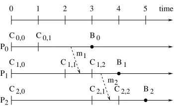
Fig. 4.1.The rollback/replay distance.
Due to nondeterminism, subsequent executions of the parallel program with the same input may not repro-duce the original bugs. This effect is called irreproducibility effect [25] or non-repeatability effect [20]. It may cause programmers confusion due to the disappearance of certain bugs and the appearance of other new bugs in repeated debugging cycles.
4.2. Record&replay methods. Record&replay methods are proposed to solve the problem of the irre-producibility effect. There are two steps in these approaches. The first step detects nondeterministic events and stores data related to them to trace files. This step is called the “record phase”. During the second step, the trace data are used as a constraint for the program, called the “replay phase”, to produce equivalent executions. Record&replay methods can be classified into two categories: data-driven [11] (or content-based/data-based [23]) and control-driven [11] (or ordering-content-based/data-based [23]). In data-driven, the contents of each message are recorded when they are received by the corresponding processes. Such a method is proposed in [4]. The biggest drawback of this technique is the requirement of significant monitor and storage overhead. Furthermore, it does not show the interactions between the different processes, and thus hinders the task of finding the cause of a bug [15]. However, it is still useful for tracing I/O or for tracing the result of certain system calls such as gettimeof day() orrandom().
The control-driven methods are based on the piecewise deterministic (PWD) execution model [26]: process execution is divided into a sequence of state intervals, each of which is started by a nondeterministic event. The execution within an interval is completely deterministic. Under the PWD assumption, execution of each deterministic interval depends only on the sequence of nondeterministic events that preceded the interval’s beginning. Thus the equivalent executions are ensured if the ordering of nondeterministic operations on all processes is the same as in the initial execution. Such an approach of control-driven technique is Instant Replay[15], which can be applied for both shared memory and message-passing programs. Following the PWD execution model, if each process is given the same input values in the same ordering during the successive executions, it will produce the same behavior each time1. Consequently, each process will produce the same
output values in the same order. These output values may then serve as input values for other processes. Therefore, we need only to trace the relative order of significant events instead of the data associated with these events. The advantage of this technique is that it requires less time and space to save the information needed for replay. Several solutions based on control-driven are implemented for both PVM programs [17] and MPI programs [2, 10].
To improve the control-driven replay technique, an optimal tracing and replay method is proposed in [20]. The key technique is that only events affecting the race conditions have to be traced. A race condition in message-passing programs occurs, if two or more messages are simultaneously to arrive at a particular receive operation and each of them can be accepted first.
4.3. Replay time and rollback/replay distance. The rollback/replay distance is introduced in [28]. The running time from evente1to evente2on the same process is called the distance betweene1ande2, denoted
d(e1, e2). The distance between global statesG1= (g1,0, g1,1, . . . , g1,n−1) andG2= (g2,0, g2,1, . . . , g2,n−1) is:
D = max(di) wheredi =d(g1,i, g2,i) and 0≤i≤n−1
Note that the definition of the distance between global statesG1andG2is only valid ifg1,i→g2,iorg1,i=
g2,i(for all i: 0≤i≤n−1), where “→” is Lamport’s “happened before” relation [14]. For example, in Fig. 4.1,
Recovery line
1
0 l
C0,0
0 l0+ l1 l0+ l + ... +ln−1 time
0
B
C m1
B1
m2
1,1
P1 P0
C1,0
Cn−1,0 Cn−1,n−1
Bn−1 mn−1
Pn−1 . . .
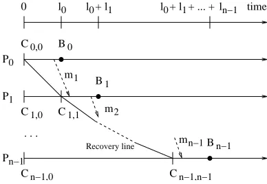
Fig. 4.2.The upper bound of the replay time.
the distance between C0,1 and B0 is 2. The distance between (C0,0, C1,1, C2,1) and (B0, B1, B2) is 3 and the
distance between (C0,1, C1,2, C2,2) and (B0, B1, B2) is 2. A relation between the rollback/replay distance and
the replay time is described in Theorem 1.
Theorem 1. If the rollback/replay distance has an upper bound L, an upper bound of the replay time is n.L, where n is number of processes.
Proof. The worst case is that each process waits for messages from another process and creates a waiting chain of processes as in Fig. 4.2. In this case, jobs are mostly executed sequentially. Thus the maximum replay time isPn−1
i=0 Li (Li is the replay distance on processPi). This value is less thann.L.
In this paper, we are interested in the distance between the recovery line and the corresponding distributed breakpoint, which is called the rollback distance or the replay distance. This replay distance is used to estimate the replay time. They are different because the replay distance is based on the previous execution while the replay time is determined during re-execution. Fig. 4.1 is an example of this difference. If users want to stop at (B0, B1, B2) while a program is recovered at (C0,0, C1,1, C2,1), then the rollback/replay distance is 3 but the
replay time is approximately 4 due to waiting of messagesm1andm2. The replay time is often larger than the
replay distance due to the required waiting of messages.
All record&replay methods described in Section 4.2 allow a parallel program to be re-executed determin-istically from the beginning state. Of course, the execution time from the beginning state to the distributed breakpoint is obviously long if the distributed breakpoint is set far from the beginning state in large-scale, long-running parallel programs. To solve this problem, checkpointing can be used. An example isIncremental Replay [31]. This replay technique uses checkpointing to allow users to run any part (checkpoint interval) of a process immediately. By using checkpointing, users do not wait for the process to run from the beginning state, thus reducing the waiting time. In addition, it also provides bounded-time in replay processes [31], which means that the replay time of a checkpoint interval does not exceed a permitted limit. Cyclic debugging is more useful when using Incremental Replay. However, Incremental Replay only supports users to replay one checkpoint interval of one process each time. (The other processes are neglected.) Each checkpoint can be seen as a breakpoint. Programmers can reach any breakpoint on a process immediately but they cannot examine the interactions between processes. In other words, Incremental Replay prohibits the use of distributed breakpoints. To minimize the waiting time during debugging, the program can be restarted at an intermediate state by using checkpointing and rollback-recovery methods. Many checkpointing and rollback-recovery methods are proposed in fault tolerance and debugging areas [1, 5, 8, 26]. However, the rollback/replay distance is still rather long in some cases [29]. It prohibits developing debugging tools, which must provide some degree of interactivity for the user’s investigations.
5. ROS-Rollback-One-Step checkpointing.
P
1 0
C
C C
C
2
P P
C0,0
1,0
2,0 2,1
0,3
Logged message (1) Recovery line
C0,1
1,2
C
2
m
0,2
C
C1,1
t2
C2,2
C1,3 (2)
(1)
(2) Distributed breakpoint
Unlogged message 2,3
C
4
m m3 m1
t1
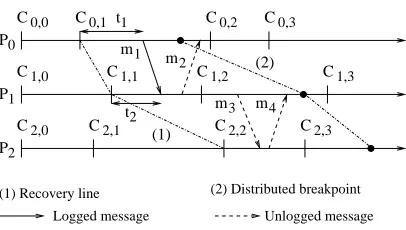
Fig. 5.1.The replay time in Rollback-One-Step (ROS).
observed during the record phase. This technique opens a possibility for minimizing the replay time in contrast to former replay techniques.
The bypassing orphan messages technique allows to minimize the rollback/replay distance between the recovery line and the corresponding distributed breakpoint. ROS ensures that an upper bound of the roll-back/replay distance is 2T [28]. Another advantage of this method is that only a small number of messages needs to be logged. Results of an implementation of this method show that the number of logged messages is mostly less than 5%, which underlines the efficiency of the logging algorithm [28].
5.2. Replay time in ROS. An upper bound of the replay distance in ROS is 2T so that an upper bound of the replay time is 2nT, where n is number of processes, following Theorem 1. The upper bound can be lowered tonT, if an additional logging rule is applied. This requires that the incoming message must be logged if the time elapsed since the last checkpoint on the send process is larger than the one on the receiving process. For example, in Fig. 5.1, messagem1 must be logged due tot1> t2. This implies that a process does not wait
for messages sent from another process if they are started at checkpoints with the same index. In addition, messages fromIp,itoIq,j withi < jare logged2so that the worst case of ROS is shown in Fig. 5.1. All processes
are rolled back one step except processP03; and if the recovery checkpoint in processPk (k >0) isCk,i, then
(1) the recovery checkpoint in processPk+1 isCk+1,i+1and (2) there is a message fromIk,i+1toIk+1,i+1, which
is not logged (messagem3in Fig. 5.1). The replay time is onlynT, where nis number of processes. In either
case, the upper bound of the replay time depends on the number of processes and thus it may be long if the number of processes is large.
6. MRT-Minimizing the Replay Time. MRT is an extension of ROS. This new method tries to keep advantages of the former method and ensures that the upper bound of the replay time is independent of the number of processes. The checkpointing techniques used in both methods are the same. This means that the state of each process is stored periodically in stable storage and the current checkpoint interval index is piggybacked on the transferred messages. When process Pp receives a message m in interval Ip,i with the
checkpoint interval indexj piggybacked on msuch that j > i, a new checkpoint with index j is immediately taken. Furthermore, the checkpoint must be placed before the receive statement.
Most important things are the rules to store the transferred messages in order to ensure that all in-transit messages of available recovery lines are logged on stable storage. In MRT, message logging is based on the following three rules:
Rule 1. Messages sent fromIq,i(i≥0) toIp,j withj > i must be logged. Rule 2. All messages sent fromIq,i−1 toIp,i−1 (i≥1) are not logged iff
(1) Cp,i→Cq,i+1, and
(2) (∀s(s6=p, q))(Cq,i→Cs,i+1)⇒(Cp,i→Cs,i+1)
Rule 3. A message from Iq,i toIp,i (i≥0) must be logged if the time elapsed since Cq,i exceeds the time
elapsed since Cp,i.
Examples of the three logging rules are shown in Fig. 6.1. Messagem1 fromI3,0toI2,1must be stored due
to Rule 1. Messagem2 fromI2,1 to I1,1 is not logged due to Rule 2, where (C1,2→C2,3)∧((C2,2 →C3,3)⇒
(C1,2 →C3,3)). But messagem3 fromI1,1 to I0,1 should be logged based on Rule 2 since ¬((C1,2→C3,3)⇒
2
This is a logging rule of ROS explained in Section 6.
P C0,0
C1,0
0
P1
P2
P3 C2,0
C3,0
I3,0
Logged message Unlogged message
C C0,3
1,3
C2,3
C3,3 C3,2
C2,2 C1,2 C0,2
3
m
2
m C1,1
3,1
C
2,1
C 1,1
I
2
t
2,1
I
4
m
m1 C0,1t1
Happened before
I0,1
Fig. 6.1. The rollback/replay distance.
P
I P
P
s
Pr
q
p
p,kp−1
Cq,kp
Cp,kp Cr,kp
r,kp−1
C
s,kp−1
C Cs,kp
q,kp−1
C
p,kp−1
C
3
m
1
m Bs
p
B
2
m
4
m
Ip,kp
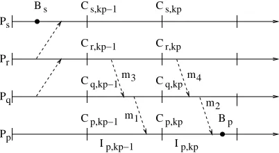
Fig. 6.2.Dependence during replaying.
(C0,2→C3,3)). Finally, messagem4 should be logged based on Rule 3 due to t1> t2. To compare MRT with
ROS, Rule 1 is kept, Rule 2 is modified, and Rule 3 is added.
Rule 1 allows recovery lines to be constructed at checkpoints with the same index because all in-transit messages of these global checkpoints are logged. It is used to avoid the domino effect [22], where cascading roll-back propagation may force the system to restart from the initial state. Obviously, the most recent checkpoints of the distributed breakpoint can be used in the corresponding recovery line by using Shortcut Replay [29]. Unfortunately, the overhead is too high because every message may become an in-transit message of an avail-able recovery line and thus it should be logged. The solution in both ROS and MRT is that each process could roll back one step during the recovery process. For instance, given an arbitrary distributed breakpoint (B0, B1, . . . , Bn−1), in which the breakpoint Bi is placed in intervalIi,ki, there always exists a corresponding
recovery line (C0, C1, . . . , Cn−1) where eitherCi =Ci,ki orCi=Ci,ki−1. To satisfy both conditions that a small
rollback distance and low message logging overhead, Rule 2 is developed. The three rules help to establish an upper bound for the replay time, which is described in Theorem 2.
Theorem 2. In MRT, there always exists a corresponding recovery line for any distributed breakpoint where - The upper bound of the replay distance is 2T, and
- The upper bound of the replay time is2T.
Proof. The proof that the upper bound of the replay distance is 2T is similar to the proof for ROS [28]. Here we prove that the upper bound of the replay time is 2T.
Consider a distributed breakpoint (B0, B1, . . . , Bn−1) (n≥2), the most recent global checkpoint
(C0,k0, C1,k1, . . . , Cn−1,kn−1)
and the corresponding recovery line
(C0,h0, C1,h1, . . . , Cn−1,hn−1)
in which (hi=ki)∨(hi=ki−1) due to the upper bound 2T of the replay distance. We prove that the replay
time fromCp,hp toBp in any processPp is less than 2T by examining the worst case in which processPp has to roll back one step, i.e. hp=kp−1. The replay time may be long due to waiting for incoming messages, such
Table 7.1 Message logging overhead.
Programs Number Execution Coordination Total Number Percentage
of processes time / time on number of of logged
checkpoint each process messages messages
interval(sec) (sec)
Message 4 19/2 0.002 120000 5507 4.59
Exchange 8 47/2 0.010 560000 15190 2.71
16 77/2 0.559 1200000 27133 2.26
Poisson 4 23/2 0.004 149866 3760 2.51
8 30/2 0.009 369084 6859 1.86
16 59/2 0.101 864078 13356 1.55
FFT 4 18/2 0.027 270024 6373 2.36
8 41/2 0.077 630056 9968 1.58
16 95/2 0.884 1350120 18458 1.37
Jacobi 4 1802/2 8.380 49924 2411 4.83
Iteration 8 510/2 1.281 73848 3032 4.11
16 268/2 2.120 153856 3442 2.24
The replay process ofIp,kp−1depends on a setψof processesPq that there exists either a direct message or a
chain of messages (a causal path), e.g. m3,m1in Fig. 6.2, fromIq,kp−1toIp,kp−1, which is not logged. It is true
that ((hq =kp−2)∨(hq=kp−1))∧(kq ≥kp−1)∧(Cq,kp−1→Cp,kp). In the case (hq =kp−2)∧(kq =kp−1),
there exists processPr(r6=p, q) such that (hr≤kp−2)∧(kr≤kp−1) and messages fromIq,kp−2 to Ir,kp−2
are not logged. Ifkr< kp−1, then Br→Bp following Rule 2 (contradiction). If (hr=kr−1)∧(kr=kp−1),
then Cr,kp−1 →Cp,kp (following Rule 2) and the recursive process is continued. The recursion is stopped at processPssuch that ((ks< kp−1)∧(Cs,kp−1→Cp,kp)) since the number of processes is finite. It also gives us
Bs→Bp (contradiction). Therefore, all processesPq inψ havehq =kp−1. Consequently, the replay time of
Ip,kp−1 is onlyT due to Rule 3.
The replay process ofIp,kp depends on a set ξ of processesPsthat there exists either a direct message or a chain of messages (a causal path), e.g. m4, m2 in Fig. 6.2, fromIs,ks to Ip,kp, which is not logged. These processesPs satisfy ((hs= kp−1)∨(hs= kp))∧(ks ≥kp). In the case that all processesPs have hs =kp,
replay time of Ip,kp is onlyT. In the others, some processesPs have (hs =kp−1)∧(ks=kp). Since replay time ofIs,ks−1 is onlyT (above proof),T could be added in the replay time ofIp,kpdue to waiting of replaying Is,ks−1. Therefore, the replay time ofIp,kp is 2T.
WhenIp,kp−1is replayed inT units time, other processesPsin ξ, which has (hs=kp−1)∧(ks=kp), are
also replayed toCs,kp during T so that replayingIp,kp requires onlyT. Therefore, the replay time in process Ppfrom Cp,hp toBp is only 2T.
7. Implementation. Checkpoints are taken periodically based on the defined checkpoint interval. How-ever, checkpoints may be taken earlier when the incoming message is from a checkpoint interval with a higher index as shown above. This section describes the method to collect data to evaluate logging rules.
Due to the checkpoint interval index piggybacked on each transferred message, it is easy to decide which messages should be logged following Rule 1. To evaluate Rule 3, an additional value must be tagged on the transferred messages. Upon sending, the timet1 elapsed since the last checkpoint is piggybacked on message
m4 as shown in Fig. 6.1. Due tot1 > t2, process P1 will save m4 to the trace files. If the incoming message
does not satisfy both Rule 1 and Rule 3, it is kept in temporary storage in order to be evaluated later based on Rule 2.
When process Pp arrives at checkpoint event Cp,i+1, it will decide to store messages received in interval
Ip,i−1 or not based on Rule 2. Of course, it requires tracking the happened-before relation between checkpoint
events. This method uses the knowledge matrix as shown in [28]. However, both processesPp at state Cp,i+1
and Pq at state Cq,i+1 cannot know accurately all processes Ps such that Cq,i → Cs,i+1. Unfortunately, the
upper bound of the replay time (and the rollback distance) in MRT will be larger than 2T if Rule 2 cannot be evaluated accurately. Only processPsat stateCs,i+1knows accurately which processPq satisfiesCq,i→Cs,i+1.
Therefore, when each process Pp arrives at state Cp,i+1, it must broadcast the information of all processes
Pr satisfyingCr,i → Cp,i+1 to all other processes and receives the same information from them. Afterwards,
0 0.5 1 1.5 2 2.5 3 3.5 4 4.5 5
0 2 4 6 8 10 12 14 16 18 20
Percentage (%)
Number of processes Message Exchange
MRT ROS
0 0.5 1 1.5 2 2.5 3 3.5 4 4.5 5
0 2 4 6 8 10 12 14 16 18 20
Percentage (%)
Number of processes Jacobi Iteration
MRT ROS
0 0.5 1 1.5 2 2.5 3 3.5 4 4.5 5
0 2 4 6 8 10 12 14 16 18 20
Percentage (%)
Number of processes Poisson
MRT ROS
0 0.5 1 1.5 2 2.5 3 3.5 4 4.5 5
0 2 4 6 8 10 12 14 16 18 20
Percentage (%)
Number of processes FFT
MRT ROS
Fig. 7.1.Percentage of the number of logged messages per the number of total messages.
The efficiency of MRT is verified through several applications, such as Message Exchange, Jacobi Iteration, FFT and Poisson, shown in Table 74. Message Exchange is a simple program in which messages are sent and
received from one process to others. Poisson is a parallel solver for Poisson’s equation. FFT performs a Fast Fourier Transformation. Jacobi Iteration is used to solve the system of linear equations. These results show that the number of logged messages is mostly less than 5% of the total number of messages. It is even better if the program’s running time is longer and does not depend on the number of processes. A comparison of the efficiency between MRT and ROS is shown in Fig. 7.1. The ratios of the number of logged messages to the total number of messages in both methods are small and each can compare with the other one.
8. The four-phase-replay method. In order to know whether to store the incoming messages for limiting the rollback distance during re-execution, the amount of monitoring must be increased. This means that more information about relations between events on processes must be obtained. Consequently, the program’s behavior may be influenced when the instrumented code slows down the execution of one or more processes. This effect is called theprobe effect[18], which is a problem in cyclic debugging since the change of a program’s behavior not only hides some errors shown in the target program’s execution but also could show additional errors. Therefore, reducing the overhead of monitoring is important.
In MRT, monitoring consists of two main parts: (1) operations at send or receive events and (2) operations at checkpoint events. The first operations help to improve the knowledge for each process about the relations between events. In order to reduce this overhead, we have to reduce both the information piggybacked on transferred messages and operations at communication events. However, it must be ensured that enough information to evaluate the three logging rules in MRT is provided. In order to collect the happened-before relation between checkpoint events on the fly, the piggybacked data on transferred messages as shown in Section 7 have been optimized.
The second operation can be evaluated through operations at each checkpoint event. This work includes (1) collecting relation between checkpoint events by a coordination among processes (See Section 7), (2) processing data and logging messages (based on Rule 2), and (3) taking a checkpoint. These are the main reasons that cause the delay in program’s execution. The problem (3) (taking a checkpoint) can be handled by means of
4
BEGIN
(very small) Instrument program
execution later) (to produce the same Store data to trace files
END Execute program
BEGIN
END Generate virtual
checkpoints
BEGIN
generate happened−
Decide messages to be logged based on Rule 2
Instrument program
Re−execute program
Instrument program BEGIN
Set breakpoint
Establish suitable recovery line
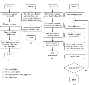
(4) The replay phase
(3) The logging&checkpointing phase (2) The evaluation phase (1) The record phase
virtual checkpoint events before relation between
(more than in phase (1))
based on the trace data Read the trace data to
END Log messages & take checkpoints Get more data of
the event graph
(2)
(1) (3)
Re−execute program
Inspect state
Bug detected?
END
(4) Yes
No based on the trace data
from the recovery line
Fig. 8.1.The four-phase-replay method.
incremental checkpointing [6] andforked checkpointing [21]. By using forked checkpointing, a child process is created and it will take a checkpoint while the main process continues its execution. In addition, only data modified in comparison with the previous checkpoint are stored in incremental checkpointing. But problems (1) and (2) cannot be solved in MRT on the fly.
To avoid the probe effect, Leu and Schiper [16], and later Teodorescu and Chassin de Kergommeaux [27] introduced a new solution, in which only minimum tracing data are required to allow re-execution of programs. Thus the initial execution is assumed to be only slightly perturbed and afterwards the replayed executions are used to collect more information. This is similar to incremental tracing [3, 12]. This idea can be applied to avoid the probe effect when using MRT.
The record&replay mechanisms with two phases are unsuitable in this case. Therefore, thefour-phase-replay method is introduced. As shown in Fig. 8.1, it has four steps as following:
1. The record phase: It requires only to collect the correct event occurrence timings in the initial execution since it is able to replay the program with clock synchronization algorithms [24]. The checkpoint events are also created in the initial execution but no checkpoint images are actually stored. Such checkpoint events are calledvirtual checkpoints. It is expected that the target program’s behavior is affected very slightly due to the small instrumentation in this step.
2. The evaluation phase: The second step is to produce the necessary information used for message logging rules in MRT. Fortunately, the direct happened-before relation between pairs of events, e.g. send and corresponding receive events of a message, is enough to exhibit the happened-before relation between virtual checkpoint events by processing off line. Hence, Rule 2 can be evaluated based on these data.
3. The logging&checkpointing phase: After executing the evaluation phase, a re-execution is required to store in-transit messages and take real checkpoints. Please note that all message logging rules in MRT can be evaluated in the logging&checkpointing phase. Of course, the re-execution in the logging&checkpointing phase will produce the same program behavior as shown in the initial execution by clock synchronization algorithms [24] and will not create serious effects.
9. Discussion. The advantage of MRT compared to ROS is the small upper bound of the replay time.(The upper bound of the replay time of ROS isnT and of EROS is 3T [30].) The disadvantage of MRT is that it requires additional synchronization mechanisms to collect data. The synchronization could produce serious probe effects due to the delay of the target program’s execution. However, the four-phase-replay method used for MRT, in which some logging rules are evaluated off line, has many advantages. First, the probe effect is avoided in this method. Monitoring can be increased in the logging&checkpointing phase to learn more about the program’s internal states. Second, the information obtained by an off-line method is more adequate than an on-the-fly method and thus the decision of logging is more accurate and efficient. For instance, the on-the-fly logging method of ROS may log messages, which are useless in replay process [28]. The reason is that a process may not obtain accurate relations between checkpoints on the fly when it decides to log messages or not based on Rule 2. This problem is solved in the four-phase-replay method since relations between checkpoints can be evaluated based on trace data.
In the future, the four-phase-replay method used for MRT will be applied in Process Isolation [12], in which users can run and inspect only a group of processes. This technique requires a re-execution to store all messages coming from the outside processes. Therefore, this step can be integrated into the logging&checkpointing phase. The resulting technique allows to reduce both the waiting time and the number of processes during debugging long-running, large-scale parallel programs [13].
10. Conclusions. A major problem that prohibits cyclic debugging with breakpointing for parallel pro-grams is the long waiting time. Although there are many efforts, the waiting time may still be rather long or the amount of trace data are too large with long-running, large-scale parallel programs. An approach to solving this problem is ROS, but its upper bound of the replay time depends on the number of processes.
The new method named MRT is shown in this paper. The upper bound of the replay time is independent of the number of processes and is only 2T at most. In addition, this method is really efficient in minimizing the number of logged messages. These characteristics are important to develop debugging tools for parallel programs, in which some degree of interactivity for the user’s investigations is required.
The disadvantage of the MRT method is that it requires coordination among processes in order to get the necessary information used in message logging. This affects not only the autonomy of each process but also synchronization between them. Consequently, the replay method is proposed. The four-phase-replay method has two advantages: (1) the process to evaluate logging rules is accurate and the message logging overhead is thus reduced, and (2) the probe effect is avoided. In addition, the four-phase-replay method can be integrated with Process Isolation in order to debug long-running, large-scale parallel programs.
Acknowledgments. We would like to thank our colleagues, especially Dieter Kranzlm¨uller, for discussions and their help to finish this paper.
REFERENCES
[1] K. M. Chandy and L. Lamport,Distributed Snapshots: Determining Global States of Distributed Systems, ACM Transac-tions on Computer Systems 3 (1985), pp. 63-75.
[2] J. Chassin de Kergommeaux, M. Ronsse and K. De Bosschere, MPL*: Efficient Record/Replay of Nondeterminism Features of Message Passing Libraries, In J. Recent Advances in Parallel Virtual Machine and Message Passing Interface (EuroPVM/MPI99) (Sept. 1999), LNCS, Springer-Verlag, Vol. 1697, pp. 141-148.
[3] J. D. Choi, B. P. Miller, R. H. B.Netzer,Techniques for Debugging Parallel Programs with Flowback Analysis, ACM Transactions on Programming Languages and Systems (Oct. 1991), Vol. 13, No. 4, pp. 491-530.
[4] R. S. Curtis, and L. D. Wittie,BugNet: A Debugging System for Parallel Programming Environments, Proc. of the 3rd Intl. Conference on Distributed Computing Systems, Miami, FL, USA (Oct. 1982), pp. 394-399.
[5] E. N. Elnozahy, L. Alvisi, Y. M. Wang and D. B. Johnson,A Survey of Rollback-Recovery Protocols in Message-Passing Systems, ACM Computing Surveys (CSUR)(Sept. 2002), Vol. 34, Issue 3, pp. 375-408.
[6] S. I. Feldman and Ch. B. Brown,Igor: A System for Program Debugging via Reversible Execution, Proc. of the ACM SIGPLAN and SIGOPS Workshop on Parallel and Distributed Debugging (May 1988), University of Wisconsin, Madison, Wisconsin, USA, SIGPLAN Notices (Jan. 1989), Vol. 24, No. 1, pp. 112-123.
[7] J. Fowler and W. Zwaenepoel,Causal Distributed Breakpoints, Proc. of the 10th International Conference on Distributed Computing Systems (ICDCS) (1990), pp. 134-141.
[8] J. M. H´elary, A. Mostefaoui and M. Raynal, Communication-Induced Determination of Consistent Snapshot, IEEE Transaction on Parallel and Distributed Systems (Sept. 1999), Vol. 10, No. 9.
[10] D. Kranzlm¨uller and J. Volkert,NOPE: A Nondeterministic Program Evaluator, Proc. of ACPC’99 (Feb. 1999), LNCS, Springer-Verlag, Vol. 1557, pp. 490-499.
[11] D. Kranzlm¨uller,Event Graph Analysis for Debugging Massively Parallel Programs, PhD Thesis, GUP Linz, Johannes Kepler University Linz, Austria (Sept. 2000),http://www.gup.uni-linz.ac.at/~dk/thesis/thesis.php.
[12] D. Kranzlm¨uller,Incremental Tracing and Process Isolation for Debugging Parallel Programs, Computers and Artificial Intelligence (2000), Vol. 19, pp. 569-585.
[13] D. Kranzlm¨uller, N. Thoai, and J. Volkert, Error Detection in Large-Scale Parallel Programs with Long Runtimes, Tools for Programs Development and Analysis (Best papers from two Technical Sessions, at ICCS2001, San Francisco, CA, USA, and ICCS2002, Amsterdam, The Netherlands), Future Generation Computer Systems (Jul. 2003), Vol. 19, No. 5, pp. 689-700.
[14] L. Lamport,Time, Clocks, and the Ordering of Events in a Distributed System, Communications of the ACM (Jul. 1978), Vol. 21, No. 7, pp. 558-565.
[15] T. J. LeBlanc and J. M. Mellor-Crummey,Debugging Parallel Programs with Instant Replay, IEEE Transactions on Computers (Apr. 1987), Vol. C-36, No. 4, pp. 471-481.
[16] E. Leu and A. Schiper,Execution Replay: A Mechanism for Integrating a Visualization Tool with a Symbolic Debugger, Proc. of CONPAR 92 - VAPP V, LNCS, Springer-Verlag (1992), Vol. 634.
[17] M. Mackey,Program Replay in PVM, Technical Report, Concurrent Computing Department, Hewlett-Packard Laboratories (May 1993).
[18] C. E. McDowell and D. P. Helmbold,Debugging Concurrent Programs, ACM Computing Surveys (Dec. 1989), Vol. 21, No. 4, pp. 593-622.
[19] Message Passing Interface Forum,MPI: A Message-Passing Interface Standard Version 1.1,http://www.mcs.anl.gov/mpi/
(Jun. 1995).
[20] R. H. B. Netzer and B. Miller,Optimal Tracing and Replay for Debugging Message-Passing Parallel Programs, Proc. of Supercomputing’92, Minneapolis, MN (Nov 1992), pp. 502-511. Reprinted in: The Journal of Supercomputing (1994), Vol. 8, No. 4, pp. 371-388.
[21] J. S. Plank,An Overview of Checkpointing in Uniprocessor and Distributed Systems, Focusing on Implementation and Performance, Technical Report UT-CS-97-372, University of Tennessee (Jul. 1997).
[22] B. Randel,System Structure for Software Fault Tolerance, IEEE Transactions on Software Engineering TSE (Jun. 1975), Vol. 1, No. 2, pp. 221-232.
[23] M. Ronsse, K. De Bosschere and J. Chassin de Kergommeaux, Execution Replay and Debugging, Proc. of the 4th International Workshop on Automated Debugging (AADEBUG2000) (Aug. 2000), pp. 5-18.
[24] Ch. Schaubschl¨ager, D. Kranzlm¨uller and J. Volkert, A Complete Monitor Overhead Removal Strategy, Proc. of PDPTA ’99, International Conference on Parallel And Distributed Processing Techniques and Applications, CSREA Press, Vol. 4, Las Vegas, Nevada, USA (Jun. 1999), pp. 1894-1897.
[25] D. F. Snelling and G. -R. Hoffmann,A Comparative Study of Libraries for Parallel Processing, Proc. of International Conference on Vector and Parallel Processors, Computational Science III, Parallel Computing (1988), Vol. 8 (1-3), pp. 255-266.
[26] R. Strom and S. Yemini,Optimistic Recovery in Distributed Systems, ACM Transactions on Computer Systems (Aug. 1985), Vol. 3, No. 3, pp 204-226.
[27] F. Teodorescu and J. Chassin de Kergommeaux,On Correcting the Intrusion of Tracing Non-deterministic Programs by Software, Proc. of EUROPAR’97 Parallel Processing, 3rd International Euro-Par Conference (Aug. 1997), LNCS, Springer-Verlag, Vol. 1300, pp. 94-101.
[28] N. Thoai, D. Kranzlm¨uller and J. Volkert,ROS: The Rollback-One-Step Method to Minimize the Waiting Time during Debugging Long-Running Parallel Programs, High Performance Computing for Computational Science, selected Papers and Invited Talks of VECPAR 2002, LNCS, Springer-Verlag, Vol. 2565, Chapter 8, pp. 664-678.
[29] N. Thoai and J. Volkert,Shortcut Replay: A Replay Technique for Debugging Long-Runnining Parallel Programs, Proc. of the Asian Computing Science Conference (ASIAN’02), Hanoi, Vietnam (Dec. 2002), LNCS, Springer-Verlag, Vol. 2550, pp. 34-36.
[30] N. Thoai, D. Kranzlm¨uller and J. Volkert, EROS: An Efficient Method for Minimizing the Replay Time based on the Replay Dependence Relation, Proc. of the 11th Euromicro Conference on Parallel, Distributed and Network-Based Processing (EUROMICRO-PDP 2003), IEEE Computer Society, ISBN 0-7695-1875-3, Genova, Italy (Feb. 2003), pp. 23-30.
[31] F. Zambonelli and R. H. B. Netzer,Deadlock-Free Incremental Replay of Message-Passing Programs, Journal of Parallel and Distributed Computing 61 (2001), pp. 667-678.
Edited by: Zsolt Nemeth, Dieter Kranzlmuller, Peter Kacsuk Received: April 4, 2003