Several conservative compact schemes for a class of nonlinear Schrödinger equations with wave operator

R E S E A R C H

Open Access

Several conservative compact schemes for

a class of nonlinear Schrödinger equations

with wave operator

Xiujun Cheng

_{and Fengyan Wu}

*_{Correspondence:}

[email protected]

1_{School of Mathematics and}

Statistics, Huazhong University of Science and Technology, Wuhan, China

2_{Center for Mathematical Sciences,}

Huazhong University of Science and Technology, Wuhan, China

Abstract

In this paper, several different conserving compact finite difference schemes are developed for solving a class of nonlinear Schrödinger equations with wave operator. It is proved that the numerical solutions are bounded and the numerical methods can achieve a convergence rate ofO(τ2_+h4_{) in the maximum norm. Moreover, by}

applying Richardson extrapolation, the proposed methods have a convergence rate ofO(τ4_+h4_{) in the maximum norm. Finally, several numerical experiments are}

presented to illustrate the theoretical results.

MSC: 65N06; 65N12

Keywords: Nonlinear Schrödinger equations with wave operator; Discrete conservation laws; Stability; Convergence

1 Introduction

This paper is concerned with the construction of several conservative compact schemes for the following generalized nonlinear Schrödinger equation (NLSE) with wave opera-tor:

utt–uxx+ iαut+β(x)f

|u|2u= 0, x∈(0,L),t∈(0,T), (1.1)

u(x, 0) =φ0(x), ut(x, 0) =φ1(x), x∈[0,L], (1.2) u(0,t) =u(L,t) = 0, t∈[0,T], (1.3)

whereu(x,t) is a complex function,αis a real constant,βandf are given real functions, and i2_{= –1. NLSE is one of the most important mathematical models with many}

applica-tions in different fields such as plasma physics [1], nonlinear optics [2–5], and bimolecular dynamics [6–8]. One remarkable feature of the model is its conservation law having the form of

E(t) =ut2L2+ux

2

L2+

L

0

β(x)F|u|2dx=E(0), (1.4)

whereF(s) =₀sf(z)dz.

In the past several years, much attention has been paid to developing effective numer-ical methods to solve the NLSE. For example, Bao and Cai [9] established uniform error estimates of finite difference methods for NLSEs with wave operator. Sun and Wang [10] investigated linearized finite difference methods for solving the NLSE. Chang et al. [11] presented several linearized finite difference schemes by applying an extrapolation tech-nique to the real coefficient of the nonlinear term. Goubet and Hamraoui [12] presented both numerical and theoretical invariability of energy and mass with finite time for two-dimensional cubic nonlinear Schrödinger equations with a radial defect. Generally speak-ing, the computational cost can be reduced by applying the linearized numerical methods. As a result, the linearized methods have been extensively investigated for many different nonlinear differential equations, e.g., [13–21]. However, the nonconservative linearized schemes may give blow-up solutions [22].

Recently, many numerical methods have been developed based on the conservation laws of (1.1). For example, Brugnano et al. [23] considered a class of energy-conserving Hamil-tonian boundary value methods for the equations. In [24], Zhang and Chang proposed a four-level explicit and conservative scheme. Wang and Zhang [25] developed some differ-ent conservative schemes based on some special techniques on the nonlinear terms. Hu and Chan [26] further considered a conservative difference scheme for two-dimensional NLSE. In [24, 26], the proposed methods have second order accuracy in spatial direc-tion. In order to improve accuracy in spatial direction, Guo et al. [27] and Cao et al. [28] introduced the energy conserving LDG methods and obtained optimal convergence or su-perconvergence of the method. Li et al. [29, 30] introduced the compact finite difference methods and investigated fully discrete numerical schemes for cubic NLSE with wave op-erator (i.e.,f(s) =s). As far as we know, there are few results on construction of conser-vative compact finite difference methods for the generalized NLSE with wave operator (1.1).

In this study, several compact finite difference schemes are developed for solving the generalized NLSE with wave operator (1.1). It is shown that the fully discrete numerical methods conserve the discrete energy. Then, the boundedness of numerical solutions and the stability of numerical methods are obtained. It is also proved that the numerical meth-ods can attain a convergence rate ofO(τ2_+h4_{) in the maximum norm. Here and below,τ}

andhare respectively the temporal and spatial stepsizes. Besides, by applying the Richard-son extrapolation algorithm, the proposed methods have a convergence rate ofO(τ4+h4) in the maximum norm. Finally, several numerical experiments are proposed to illustrate all the theoretical results.

The rest of the paper is organized as follows. In Sect. 2, a compact difference scheme is given. In Sect. 3, the discrete conservation law of the compact scheme is obtained. In Sect. 4, the boundedness of numerical solutions is obtained. In Sect. 5, stability and con-vergence are proved. In Sect. 6, several conservative compact schemes are constructed for the nonlinear Schrödinger equation with wave operator. Moreover, the Richardson ex-trapolation technique is used. In the last section, numerical experiments are presented to support theoretical results.

2 Finite difference scheme

Letτ=T

N andh= L

J be the temporal and spatial stepsizes, respectively, whereJandNare

given positive integers. Denotetn=nτ(0≤n≤N),xj=jh(0≤j≤J),τ ={tn|0≤n≤N},

andh={xj|0≤j≤J}. LetWh0={wnj|wn0=wnJ = 0,j= 1, 2, . . . ,J– 1,n= 1, . . . ,N– 1}be a

grid function space defined onh×τ. Define

δxwnj =

wn j+1–wnj

h , δx¯w

n j =

wn j –wnj–1

h ,

δ2_xwn_j =δxδx¯wnj =

1

h2

wn_j+1– 2wn_j +wn_j–1,

δˆtwnj =

wn_j+1–wn_j–1

2τ , δ¯tw n j =

wn_j –wn_j–1

τ , δtwnj =

wn+1

j –wnj τ , δ2_twn_j =δtδ¯twnj =

1

τ2

wn_j+1– 2wn_j +wn_j–1,

Ahwnj =

1 12

wn_j–1+ 10wn_j +wn_j+1,

wn, vn=h

J–1

j=1

wn_jv¯n_j, wn=

_hJ–1

j=1

wn j

2

,

δxwn= _hJ–1

j=0

δxwnj

2

, wn_∞= max

1≤j≤J–1

wn_j,

(2.1)

where wn_{= (w}n

1, . . . ,wnJ–1)T, vn= (vn1, . . . ,vnJ–1)T.

At the grid point (xj,tn), we define Ujnas the exact solution andunj as the numerical

solution. We also assume that the exact solution of problem (1.1)–(1.3) satisfies

maxUn,δxUn,Un_∞

≤C.

Now, we present a compact difference scheme for problem (1.1)–(1.3) as follows:

Ahδ2tunj –δ2xujn+ iαAhδˆtunj +Ah

β(xj)

F(|un+1

j |2) –F(|unj–1|2)

|un_j+1|2_–|un–1

j |2

un+1

j +unj–1

2

= 0, 1≤j≤J– 1, 1≤n≤N– 1, (2.2)

u0_j =φ0(xj), δˆtu(xj, 0) =φ1(xj), 0≤j≤J, (2.3)

un₀=un_J = 0, 0≤n≤N. (2.4)

Denote

un=un₁, . . . ,un_J–1T,

Gun2=diag

β(x1)

F(|un₁+1|2) –F(|un₁–1|2)

|un₁+1|2_–|_un–1

1 |2

, . . . ,β(xJ–1) F(|un+1

J–1|2) –F(|unJ–1–1|2) |un_J–1+1|2_–|_un–1

J–1|2

T

S=

⎛ ⎜ ⎜ ⎜ ⎜ ⎜ ⎜ ⎜ ⎝

0 1 0 . . . 0 0 1 0 1 . . . 0 0

..

. ... ... ... ... 0 0 0 . . . 0 1 0 0 0 . . . 1 0

⎞ ⎟ ⎟ ⎟ ⎟ ⎟ ⎟ ⎟ ⎠

(J–1)×(J–1)

, (2.5)

M= 1

12(10I + S), A= 1

h2(–2I + S), (2.6)

where I is an identity matrix.

Since M is a symmetric positive definite matrix, there exists a real symmetric positive definite matrix H such that H = M–1_{. Then scheme (2.2)–(2.4) can be written in the}

fol-lowing vector form:

δ2_tun– HAun+ iαδ_ˆtun+Gun2u

n+1_{+ u}n–1

2 = 0, 1≤n≤N– 1, (2.7)

u0_j =φ0(xj), δˆtuj0=φ1(xj), 0≤j≤J, (2.8)

un₀=un_J = 0, 0≤n≤N. (2.9)

3 Discrete conservation law

In this section, we will show that the numerical scheme owns the discrete conservation law. First of all, we introduce some lemmas, which will assist a lot in the proof of the main result.

Lemma 3.1(cf. [31]) The eigenvaluesλj_Sof matrixSare2cos(jπ_J ) (j= 1, 2, . . . ,J– 1).Then the eigenvalues of matricesH, A,andHAare 12

10+λj_S,

–2+λj_S

h2 ,

12(–2+λj_S)

h2_(10+λj

S)

(j= 1, 2, . . . ,J– 1), re-spectively.

Lemma 3.2 For any mesh functionu∈W_h0and real symmetric positive definite matrices

HandA,we obtain that–HAis a symmetric positive definite matrix and

–(HAu, u) =Ru2, (3.1)

whereRis obtained by Cholesky decomposition for–HA,denoted asR=Chol(–HA).

Proof It follows from M =₁₂1(10I + S) and A =_h12(–2I + S) that

MA= 1

12h2(10I + S)(–2I + S) =

1 12h2

–20I + 8S + S2= AM.

Therefore, AH = HA, which implies that (–AH)T_{= –AH.}

In virtue of Lemma 3.1, we can obtain

0≤λj_–HA= –12(–2 +λ

j S)

h2_{(10 +λ}j

S)

≤ 6

h2 (j= 1, 2, . . . ,J– 1).

Define

En=δtun

2

+1 2Ru

n2_+Run+12_–τ2

2 Rδtu

n2

+h 2

J–1

j=1

βj

Fun_j2+Fun_j+12. (3.2)

Then we get the following energy preserving property for the fully discrete numerical scheme (2.7)–(2.9).

Theorem 3.3 The numerical solutions obtained by the fully discrete numerical scheme

(2.7)–(2.9)admit:for all n≥0,En_=E0_.

Proof Taking the inner product on both sides of (2.7) with un+1_{– u}n–1_{and considering the}

real part, we arrive at

Reδ2_tun, un+1– un–1=δtun

2

–δtun–1

2

, (3.3)

ReHAun, un+1– un–1 = –1

2Ru

n+12

–Run–12+τ

2

2Rδtu

n2

–Rδtun–12

, (3.4)

Reiαδ_ˆtun, un+1– un–1= 0, (3.5)

Re

Gun2u

n+1_{+ u}n–1

2 , u

n+1_{– u}n–1

=h 2

J–1

j=1

βj

Fun_j+12–Fun_j–12. (3.6)

From (3.3)–(3.6), we have

δtun2–δtun–12+

1 2Ru

n+12

–Run–12

–τ

2

2Rδtu

n2

–Rδtun–12

+h 2

J–1

j=1

βj

Fun_j+12–Fun_j–12= 0,

which further implies that, forn≥1,

En=En–1.

Therefore, the conclusion holds.

4 Boundedness of numerical solutions

Lemma 4.1(see [32]) For any mesh functionu, v∈W_h0,there is the identity

–h

J–1

j=1

δ2_xuj

¯ vj=h

J–1

j=0

(δxuj)(δxv¯j),

which implies that–(Au, u) =δxu2.

Lemma 4.2(cf. [33]) For any symmetric matrixN,the property of Rayleigh–Ritz ratio is

min[λN]≤

(Nx, x)

(x, x) ≤max[λN],

where(x, y)indicates the inner product ofxandy,min[λN]andmax[λN]denote the

small-est and largsmall-est eigenvalue of matrixN,respectively.

Lemma 4.3 For any mesh functionu∈W0

h,it holds that–(Au, u)≤–(HAu, u).That is,

δxu ≤ Ru.

Proof It follows from HA = AH and AT_{= A that A – AH is a symmetric matrix. According}

to Sx=λj_Sx, we obtain

Hx= 12

10 +λj_Sx, Ax=

1

h2

–2 +λj_Sx. (4.1)

Therefore,

(I – H)x=

1 – 12 10 +λs_j

x= 1

h2

1 – 12 10 +λj_S

–2 +λj_SA–1x. (4.2)

Then the eigenvalues of A – AH are given by (–2+λ

j S)2

h2_(10+λj

S)

. As a result, A – AH is a symmetric and positive definite matrix.

Further, for u∈W0

h, we get uT(A – AH)u≥0, which completes the proof. Lemma 4.4(cf. [24]) For any mesh functionun_∈W0

h,there is un+12–un2≤τδtun

2

+1 2u

n2

+un+12.

Lemma 4.5(Discrete Sobolev’s inequality [34]) Suppose that{uj}is mesh functions.Given > 0,there exists a constant C dependent onsuch that

u_∞≤δxu+Cu.

Lemma 4.6 Suppose thatφ0∈H01,φ1∈L2,β(x)≥0,F(s)≥0,s∈[0, +∞),β,f∈C1(R), andτ2

h2 <1₃.Then the following estimates hold:

Proof It follows from Theorem 3.3 that there exists a constantCsuch that

En=δtun

2

+1 2Ru

n2_+Run+12_–τ2

2 Rδtu

n2

+h 2

J–1

j=1

βj

Fun_j2+Fun_j+12=C. (4.4)

Applying Lemma 3.1 and Lemma 4.2, we can deduce that

–τ

2

2 Rδtu

n2_≥

–3τ

2

h2 δtu

n2

. (4.5)

Substituting (4.5) into (4.4), we obtain that

δtun

2

+1 2Ru

n+12_+Run2_–3τ2

h2 δtu

n2_{≤C. (4.6)}

Furthermore, inequality (4.6) can be rewritten as

1 –3τ

2

h2

δtun

2

+1 2Ru

n+12_+Run2_{≤C. (4.7)}

Noting that (1 –3_hτ22) > 0, we have

δtun≤C, Run≤C.

Applying Lemma 4.4 to δtun ≤C, we obtain un ≤C. Using Lemma 4.3, we have

δxun ≤C. Moreover, by Lemma 4.5, it holds that un_∞≤C.

Therefore, the proof is completed.

5 Convergence and stability of the difference scheme

In this section, we focus on the convergence and stability of the numerical scheme. Firstly, we define the truncation errorErn

j as

Ern_j =δ2_tU_jn–A_h–1δ_x2U_jn+ iαδˆtUjn

+

β(xj)

F(|U_jn+1|2) –F(|U_jn–1|2)

|U_jn+1|2_–|_Un–1

j |2

U_jn+1+U_jn–1

2

. (5.1)

By Taylor’s expansion, it is easy to check that

Ern_j≤Cτ2+h4.

Lemma 5.1(Discrete Gronwall’s inequality [35]) Suppose that the discrete function wn

satisfies the recurrence formula

wn–wn–1≤aτwn+bτwn–1+cnτ,

where a,b and cn(n= 1, . . . ,N)are nonnegative constants.Then

max

1≤n≤N|wn| ≤

w0+τ

N

k=1 ck

e2(a+b)T,

whereτ is small such that(a+b)τ≤N_2N–1(N> 1).

Theorem 5.2 Suppose thatφ0∈H01,φ1∈L2,β(x)≥0,F(s)≥0,s∈[0, +∞),β,f∈C1(R), and τ_h22 <1₃,then the solution unof difference problem(2.7)–(2.9)converges to the solution

of problem(1.1)–(1.3)with orderO(τ2+h4)in the maximal norm.

Proof Let Ern= (Ern

1, . . . ,ErnJ–1)Tand en= Un– un. Firstly, subtracting (2.2) from the vector

form of (5.1), the error equations satisfy

Ern=δ2_ten– HAen+ iαδ_ˆten+GUnU

n+1_{+ U}n–1

2 –G

unu

n+1_{+ u}n–1

2 =δ2_ten– HAen+ iαδ_ˆten+GUne

n+1_{+ e}n–1

2 +GUn–Gunu

n+1_{+ u}n–1

2 . (5.2)

Computing the inner product with both sides of (5.2) withδ_ˆtenand considering the real part, we obtain

ReErn,δtˆen

= 1 2τδte

n2_–δ ten–1

2

+ 1 4τRe

n+12_–Ren–12

–τ 4Rδte

n2_–Rδ ten–1

2

+Re

GUne

n+1_{+ e}n–1

2 ,δˆte

n

+ReGUn–Gunu

n+1_{+ u}n–1

2 ,δˆte

n

. (5.3)

Noticing that|G(Un_{)| ≤Candf(s)∈C}1_{, we have}

ReErn,δ_tˆen≤CErn2+δten2+δten–12

, (5.4)

Re

GUne

n+1_{+ e}n–1

2 ,δˆte

n

≤Cen+12+en–12+δten2+δten–12

, (5.5)

ReGUn–Gunu

n+1_{+ u}n–1

2 ,δˆte

n

≤Cδten

2

+δten–1

2

+en2. (5.6)

It follows from Lemma 4.4 that 1

τe

n2_–en–12_≤Cδ

ten–1

2

Substituting (5.4)–(5.6) into (5.3) and combining with (5.7), we obtain 1

2τδte n2

–δten–12

+ 1 4τRe

n+12

–Ren–12

+1

τe

n2_–en–12_–τ

4Rδte

n2_–Rδ ten–1

2

≤CErn2+δten

2

+δten–1

2

+en+12+en2+en–12. (5.8)

Summing inequalities (5.8) up fornleads to

δten

2

+1 2Re

n+12_+Ren2_{+ 2e}n2_–τ2

2 Rδte

n2

≤τC

n

i=1

δtei

2

+1 2Re

i+12

+Rei2+ 2ei2

–τ

2

2 Rδte

i2

+CTτ2+h42. (5.9)

According to Lemma 5.1, it yields that

δten2+

1 2Re

n+12

+Ren2+ 2en2–τ

2

2 Rδte

n2

≤CTτ2+h42. (5.10)

Moreover, combining inequality (4.5) and using Lemma 4.2, we get

1 –3τ

2

h2

δten2+

1 2Re

n+12

+Ren2+ 2en2

≤CTτ2+h42. (5.11)

The rest of the proof of convergence is similar to that of Theorem 4.6. As a result, we have

en_∞≤Oτ2+h4. (5.12)

The proof is completed.

Similarly, we present the stability of difference scheme (2.7)–(2.9).

Theorem 5.3 Under the conditions of Theorem5.2,the difference scheme(2.7)–(2.9)is stable for the initial data.

6 Some extensions

6.1 Several conservative compact schemes

In this subsection, the proofs of the boundedness of numerical solutions, the stability and convergence of numerical schemes are similar to those in the previous sections. We only list the numerical schemes and the discrete energy conservative laws for all schemes.

Scheme1

Ahδ2tunj –δ2x

un+1

j +unj–1

2 + iαAhδˆtu

n j

+Ah

β(xj)

F(|un_j+1|2) –F(|un_j–1|2)

|un_j+1|2_–|_un–1

j |2

un_j+1+un_j–1

2

= 0,

1≤j≤J– 1, 1≤n≤N– 1,

u0_j =φ0(xj), δˆt(xj, 0) =φ1(xj), 0≤j≤J,

un

0=unJ = 0, 0≤n≤N.

The discrete conservative law of Scheme 1 is

En=δtun

2

+1 2Ru

n2

+Run+12+h 2 J–1 j=1 βj

Fun_j2+Fun_j+12=E0.

Scheme2

Ahδ2tunj –δ2x

un+1

j +unj–1

2 + iαAhδˆtu

n j

+Ah

β(xj)

F(|u

n+1

j |2+|unj|2

2 ) –F(

|un j|2+|unj–1|2

2 )

|un+1

j |2–|unj–1|2

un_j+1+un_j–1= 0,

1≤j≤J– 1, 1≤n≤N– 1,

u0_j =φ0(xj), δˆt(xj, 0) =φ1(xj), 0≤j≤J,

un₀=un_J = 0, 0≤n≤N.

The discrete conservative law of Scheme 2 is

En=δtun

2

+1 2Ru

n2

+Run+12+h

J–1

j=1

βjF _|un+1

j |2+|unj|2

2

=E0.

Scheme3

Ahδ2tunj –δ2xunj + iαAhδˆtunj

+Ah

β(xj)

F(|u

n+1

j |2+|unj|2

2 ) –F(

|un_j|2+|un_j–1|2

2 )

|un+1

j |2–|unj–1|2

un_j+1+un_j–1= 0,

1≤j≤J– 1, 1≤n≤N– 1,

u0_j =φ0(xj), δˆt(xj, 0) =φ1(xj), 0≤j≤J,

The discrete conservative law of Scheme 3 is

En_=δ tun

2

+1 2Ru

n2_+Run+12_–τ2

2 Rδtu

n2

+h

J–1

j=1

βjF _|un+1

j |2+|unj|2

2

=E0.

Scheme4

Ahδ2t

un_j+1+un_j

2 –δ

2

x

un_j+1+un_j

2 + iαAhδtu

n j

+Ah

β(xj)

F(|un+1

j |2) –F(|unj|2)

|un_j+1|2_–|_un j|2

un+1

j +unj

2

= 0,

1≤j≤J– 1, 1≤n≤N– 1,

u0_j =φ0(xj), δˆt(xj, 0) =φ1(xj), 0≤j≤J,

un₀=un_J = 0, 0≤n≤N.

The discrete conservative law of Scheme 4 is

En=1 2δtu

n2_+δ ¯ tun

2

–τ

2

2δ

2

tun

2

+Run2+h

J–1

j=1

βjFunj

2

=E0.

6.2 Richardson extrapolation

In order to improve the accuracy in the temporal direction, we apply Richardson ex-trapolation, which is given by a linear combination of numerical solutions under dif-ferent mesh grids. Applying Taylor’s expansion, we obtain that the main term of trun-cation error Ern_j isO(τ2+τ4 +h4). Hence, we use the following Richardson method (see [36]):

(uR)nj =

4 3u

2n j

h,τ 2

–1 3u

n j(h,τ),

whereun_j(h,τ) is the numerical solutions at the grid point (xj,tn) with spatial step sizehand

temporal step sizeτ, andu2n

j (h,τ2) is the numerical solutions at the grid point (xj,tn) with

spatial step sizehand temporal step sizeτ₂. Here, the convergence order of the Richardson method isO(τ4+h4_).

7 Numerical experiments

In this section, we use serval numerical experiments to confirm the discrete conservation law, convergence as well as stability. Due to the implicitness and nonlinearity in scheme (2.7)–(2.9), the split iterative algorithm [37] is used to resolve this problem. We take 10–8

Example1 We present some accuracy tests by considering the following equation:

utt–uxx+ iut+|u|4u=f(x,t), (x,t)∈(0, 1)×(0, 1), (7.1)

u(x, 0) =x(x– 1), ut(x, 0) = –ix(x– 1), x∈[0, 1], (7.2)

u(0,t) =u(1,t) = 0, t∈[0, 1], (7.3) wheref(x,t) = –2e–it_+x5_{(x– 1)}5_e–it_.

The exact solution of the problem is

u(x,t) =e–it(x– 1)x.

In this example, the maximum norm is defined as follows:

err1∞= max

0≤j≤J

0≤n≤N

u(xj,tn) –unj,

errR1∞= max

0≤j≤J

0≤n≤N

u(xj,tn) –

4 3u

2n j

h,τ 2

–1 3u

n j(h,τ)

.

Scheme (2.7)–(2.9) withτ =h2is applied to solve (7.1)–(7.3). The numerical errors are plotted in Fig. 1. It indicates that the convergence order of the scheme isO(τ2+h4_{). To}

improve temporal accuracy, Richardson extrapolation withτ =his applied to solve the problem. The numerical errors are given in Fig. 2. Clearly, it implies that the convergence

Figure 1The convergence order of scheme (2.7)–(2.9) for Example 1

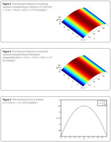
Figure 3The long-term behavior of numerical solutions corresponding to scheme (2.7)–(2.9) from

t= 0 tot= 10 ath= 0.01,τ=h2for Example 1

Figure 4The long-term behavior of numerical solutions corresponding to Richardson

extrapolation fromt= 0 tot= 10 ath= 0.01,τ=h2

for Example 1

Figure 5The movement of|u|of scheme (2.7)–(2.9) att= 2, 5, 10 for Example 1

order of the method isO(τ4_+h4_{). We also numerically solve the problem withh= 0.01,}

τ =h2_{, andT = 10. Figs. 3 and 4 indicate the long-term behavior of numerical solutions}

with respect to scheme (2.7)–(2.9) and Richardson extrapolation, respectively. Figs. 5 and 6 further show the movement of|u|at different times, i.e.,t= 2, 5, 10. These figures further imply that the numerical schemes are effective.

Example2 In order to further confirm the theoretical results, we present the following tests by considering the following equation:

utt–uxx+ iut+|u|2u= 0, (x,t)∈(–40, 40)×(0, 1),

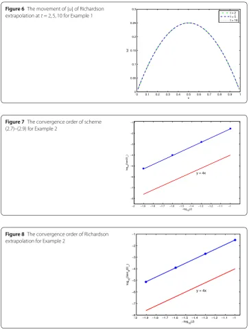
Figure 6The movement of|u|of Richardson extrapolation att= 2, 5, 10 for Example 1

Figure 7The convergence order of scheme (2.7)–(2.9) for Example 2

Figure 8The convergence order of Richardson extrapolation for Example 2

The maximum norm in this test is defined as follows:

err2∞= max

0≤j≤J

0≤n≤N

u(xj,tn) –unj,

errR2∞= max

0≤j≤J

0≤n≤N

u(xj,tn) –

4 3u

2n j

h,τ 2

–1 3u

n j(h,τ)

.

Figure 9The wave propagation of scheme (2.7)–(2.9) ath= 0.1,τ=h2for Example 2

Figure 10 The wave propagation of Richardson extrapolation ath= 0.1,τ=h2for Example 2

Figure 11 The movement of|u|of scheme (2.7)–(2.9) att= 2, 5, 10 for Example 2

results indicate that the convergence order of scheme (2.7)–(2.9) isO(τ2_+h4_{) and the}

convergence order of the scheme with Richardson extrapolation isO(τ4+h4_{). Moreover,}

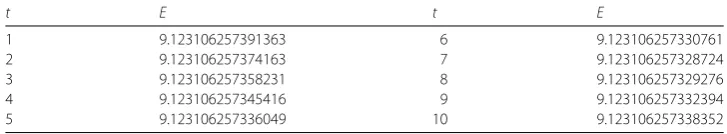
Figs. 9 and 10 display the wave propagation of scheme (2.7)–(2.9) and Richardson extrap-olation with h= 0.1,τ =h2, andT = 10, respectively. Figs. 11 and 12 show the move-ment of|u|of scheme (2.7)–(2.9) and Richardson extrapolation att= 2, 5, 10, respectively. In order to further confirm the discrete conservation law, we chooseh= 0.05,τ =h2_to

Figure 12 The movement of|u|of Richardson extrapolation att= 2, 5, 10 for Example 2

Table 1 The discrete energyEat different time withh= 0.05,τ=h2for Example 2

t E t E

1 9.123106257391363 6 9.123106257330761

2 9.123106257374163 7 9.123106257328724

3 9.123106257358231 8 9.123106257329276

4 9.123106257345416 9 9.123106257332394

5 9.123106257336049 10 9.123106257338352

8 Conclusion

In this work, we presented several conservative compact schemes for solving a class of nonlinear Schrödinger equations with wave operator. By the energy method, it was proved that the numerical solution is bounded and numerical scheme (2.7)–(2.9) is convergent and stable. The convergence rate isO(τ2+h4_{) inl}

∞ norm. Furthermore, the order of

scheme (2.7)–(2.9) is improved toO(τ4+h4_{) by applying Richardson extrapolation.}

Fi-nally, all the numerical results show that difference scheme (2.7)–(2.9) and Richardson extrapolation are efficient.

Acknowledgements

We would like to thank Prof. Jinqiao Duan and Dr. Xiaoli Chen for helpful discussions.

Funding

This work was partly supported by the National Science Foundation (grant No. 1620449) and the National Natural Science Foundation of China (grant Nos. 11771162, 11531006, and 11771449).

Availability of data and materials

Not applicable.

Competing interests

All authors declare that none of them has competing interests.

Authors’ contributions

XC designed the numerical schemes and wrote the first draft of the manuscript. FW considered the numerical simulations. Both authors read and approved the final version of the manuscript.

Publisher’s Note

Springer Nature remains neutral with regard to jurisdictional claims in published maps and institutional affiliations.

Received: 4 December 2017 Accepted: 12 March 2018 References

2. Schoene, A.Y.: On the nonrelativistic limits of the Klein–Gordon and Dirac equations. J. Math. Anal. Appl.71, 36–47 (1979)

3. Bergé, L., Colin, T.: A singular perturbation problem for an envelope equation in plasma physics. Physica D84, 437–459 (1995)

4. Liao, L., Ji, G., Tang, Z., Zhang, H.: Spike-layer simulation for steady-state coupled Schrödinger equations. East Asian J. Appl. Math.7, 566–582 (2017)

5. Saanouni, T.: Global well-posedness of some high-order focusing semilinear evolution equations with exponential nonlinearity. Adv. Nonlinear Anal.7, 67–84 (2017)

6. Xin, J.: Modeling light bullets with the two-dimensional sine-Gordon equation. Physica D135, 345–368 (2000) 7. Guo, B., Hua, H.: On the problem of numerical calculation for a class of the system of nonlinear Schrödinger equation

with wave operator. J. Numer. Methods Comput. Appl.4, 258–263 (1983)

8. Holzleitner, M., Kostenko, A., Teschl, G.: Dispersion estimates for spherical Schrödinger equations: the effect of boundary conditions. Opusc. Math.36(6), 769–786 (2016)

9. Bao, W., Cai, Y.: Uniform error estimates of finite difference methods for the nonlinear Schrödinger equation with wave operator. SIAM J. Numer. Anal.50, 492–521 (2012)

10. Sun, W., Wang, J.: Optimal error analysis of Crank–Nicolson schemes for a coupled nonlinear Schrödinger system in 3D. J. Comput. Appl. Math.317, 685–699 (2017)

11. Chang, Q., Jia, E., Sun, W.: Difference schemes for solving the generalized nonlinear Schrödinger equation. J. Comput. Phys.148, 397–415 (1999)

12. Goubet, O., Hamraoui, E.: Blow-up of solutions to cubic nonlinear Schrödinger equations with defect: the radial case. Adv. Nonlinear Anal.6(2), 183–197 (2017)

13. Li, D., Wang, J.: Unconditionally optimal error analysis of Crank-Nicolson Galerkin FEMs for a strongly nonlinear parabolic system. J. Sci. Comput.72, 892–915 (2017)

14. Li, D., Zhang, C., Ran, M.: A linear finite difference scheme for generalized time fractional Burgers equation. Appl. Math. Model.40, 6069–6081 (2016)

15. Li, D., Liao, H., Sun, W., Wang, J., Zhang, J.: Analysis of L1-Galerkin FEMs for time-fractional nonlinear parabolic problems. Commun. Comput. Phys.24, 86–103 (2018)

16. Jannelli, A., Ruggieri, M., Speciale, M.P.: Exact and numerical solutions of time-fractional advection-diffusion equation with a nonlinear source term by means of the Lie symmetries. Nonlinear Dyn. (2018).

https://doi.org/10.1007/s11071-018-4074-8

17. Zhang, Q., Zhang, C., Wang, L.: The compact and Crank–Nicolson ADI schemes for two-dimensional semilinear multidelay parabolic equations. J. Comput. Appl. Math.306, 217–230 (2016)

18. Zhang, Q., Mei, M., Zhang, C.: Higher-order linearized multistep finite difference methods for non-Fickian delay reaction-diffusion equations. Int. J. Numer. Anal. Model.14, 1–19 (2017)

19. Li, D., Wang, J., Zhang, J.: Unconditionally convergentL1-Galerkin FEMs for nonlinear time-fractional Schrödinger equations. SIAM J. Sci. Comput.39, A3067–A3088 (2017)

20. Li, D., Zhang, J., Zhang, Z.: Unconditionally optimal error estimates of a linearized Galerkin method for nonlinear time fractional reaction-subdiffusion equations. J. Sci. Comput. (2018). https://doi.org/10.1007/s10915-018-0642-9 21. Kumar, S., Kumar, D., Singh, J.: Fractional modelling arising in unidirectional propagation of long waves in dispersive

media. Adv. Nonlinear Anal.5(4), 383–394 (2016)

22. Zhang, F., Peréz-Ggarcía, V.M., Vázquez, L.: Numerical simulation of nonlinear Schrödinger equation system: a new conservative scheme. Appl. Math. Comput.71, 165–177 (1995)

23. Brugnano, L., Zhang, C., Li, D.: A class of energy-conserving Hamiltonian boundary value methods for nonlinear Schrödinger equation with wave operator. Commun. Nonlinear Sci. Numer. Simul.60, 33–49 (2018)

24. Zhang, L., Chang, Q.: A conservative numerical scheme for a class of nonlinear Schrödinger equation with wave operator. Appl. Math. Comput.145, 602–613 (2003)

25. Wang, T., Zhang, L.: Analysis of some new conservative schemes for nonlinear Schrödinger equation with wave operator. Appl. Math. Comput.182, 1780–1794 (2006)

26. Hu, H., Chan, Y.: A conservative difference scheme for two-dimensional nonlinear Schrödinger equation with wave operator. Numer. Methods Partial Differ. Equ.32, 862–876 (2016)

27. Guo, L., Xu, Y.: Energy conserving local discontinuous Galerkin methods for nonlinear Schrödinger equation with wave operator. J. Sci. Comput.65, 622–647 (2015)

28. Cao, W., Li, D., Zhang, Z.: Optimal superconvergence of energy conserving local discontinuous Galerkin methods for wave equations. Commun. Comput. Phys.21, 211–236 (2017)

29. Li, X., Zhang, L., Wang, S.: A compact finite difference scheme for the nonlinear Schrödinger equation with wave operator. Appl. Math. Comput.219, 3187–3197 (2012)

30. Li, X., Zhang, L., Zhang, T.: A new numerical scheme for the nonlinear Schrödinger equation with wave operator. Appl. Math. Comput.54, 109–125 (2017)

31. Li, D., Zhang, C., Wen, J.: A note on compact finite difference method for reaction-diffusion equations with delay. Appl. Math. Model.39, 1749–1754 (2015)

32. Sun, Z.: Numerical Methods of the Partial Differential Equations. Science Press, Beijing (2005) 33. Horn, R.A., Johnson, C.R.: Matrix Analysis. Cambridge University Press, Cambridge (2012)

34. Chan, T., Shen, L.: Stability analysis of difference schemes for variable coefficient Schrödinger type equations. SIAM J. Numer. Anal.24, 336–349 (1981)

35. Zhou, Y.: Application of Discrete Functional Analysis to the Finite Difference Methods. International Academic Publishers, Beijing (1990)

36. Deng, D., Zhang, C.: Analysis and application of a compact multistep ADI solver for a class of nonlinear viscous wave equations. Appl. Math. Model.39, 1033–1049 (2015)