R E S E A R C H
Open Access
Schauder’s fixed-point theorem: new
applications and a new version for
discontinuous operators
Rodrigo López Pouso
**Correspondence:
[email protected] Departamento de Análise Matemática, Facultade de Matemáticas, Universidade de Santiago de Compostela, Campus Sur, Santiago de Compostela, 15782, Spain
Abstract
Schauder’s fixed-point theorem, which applies for continuous operators, is used in this paper, perhaps unexpectedly, to prove existence of solutions to discontinuous problems. Moreover, we introduce a new version of Schauder’s theorem for not necessarily continuous operators which implies existence of solutions for wider classes of problems. Leaning on an abstract fixed-point theorem, our approach is not limited to one-dimensional homogeneous Dirichlet problems, the only type of examples worked out in this paper for coherence and simplicity but yet novelty.
MSC: 47H10; 34A36; 34B15
Keywords: Schauder’s theorem; fixed-point theorem; discontinuous differential equations
1 Introduction
This paper contains a probably unexpected application of Schauder’s fixed-point theorem to a class of discontinuous problems, and a generalization of it that we have never seen before and proves useful in even more general contexts.
Our new version of Schauder’s theorem yields novel existence results even for thor-oughly studied problems such as
x=f(t,x), x() =x() = , (.)
with aL-bounded nonlinearityf. The importance of our abstract result is that it allows f to be discontinuous with respect to the dependent variable and does not lean on mono-tonicity at all. This is a significant contribution to the available literature on existence of solutions to (.) with discontinuousf’s which, roughly speaking, consists in rewriting f(t,x) =g(t,x,x) for some functiongwhich is continuous with respect to its second argu-ment and monotone nonincreasing with respect to the third one. Essential references for this approach are [, ], and some more recent related results can be looked up in [, , , ].
Removing assumptions from the basic theory on (.) can only be useful in applications. Motions of particles in a force field, stationary distributions of temperatures, and many other phenomena can be modeled by means of equations of the formx=f(t,x). In real life, external forcesf(t,x) often assume only a discrete set of more than one value, so they are often discontinuous (and not necessarily monotone).
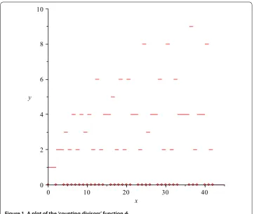
Figure 1 A plot of the ‘counting divisors’ functionφ.
For completeness and later references, let us recall Schauder’s theorem [, Theo-rem ..].
Schauder’s Fixed-Point Theorem Let K be a nonempty, convex, and compact subset of a normed space.
Any continuous operator T:K–→K has at least one fixed point.
In order to illustrate our new application of Schauder’s theorem, we shall construct some examples based on the following discontinuous and nonmonotone function: let us call
φ(x) the number of divisors of the integer part ofx∈[, +∞). See Figure for a plot of this function.
Obviously,φ is piecewise constant, discontinuous at infinitely many natural numbers, right-continuous at everyx≥,φ(x)≥ for allx≥, and
lim sup
x→+∞
φ(x) = +∞.
There exist arbitrarily big prime numbers, so we also have
lim inf
x→+∞φ(x) = .
Proposition . There exists at least one solution in W,(, )to the Dirichlet problem
x= φ
√
t+|x|
for almost all t∈[, ], x() =x() = , (.)
whereφ(z)is the number of divisors of the integer part of z∈[, +∞).
Notice that the right-hand side of the differential equation in (.) has discontinuities with respect to the unknown in every neighborhood of the boundary condition (t,x) =
(, ). This makes it surprising at first sight that Schauder’s theorem can be applied. The rest of this paper is organized as follows. In Section , we show how to apply Schauder’s theorem to derive a pretty easy proof of existence of solutions for a class of discontinuous second-order scalar problems containing (.) as a particular case. While our existence result in Section is quite general and has an easy proof, it is somewhat re-stricted in the type of discontinuities that it admits. In Section , we present a generaliza-tion of Schauder’s theorem for not necessarily continuous operators which allows working with more general types of discontinuities, as we illustrate in Section . Our fixed-point type approach is not limited to second-order differential equations or to homogeneous Dirichlet conditions, which we have considered only for the sake of simplicity.
2 A new application of Schauder’s theorem
One of the simplest and best known applications of Schauder’s fixed-point theorem is the proof of existence of solutions to
x=f(t,x) for a.a.t∈I= [, ], x() =x() = , (.)
under the so-called Carathéodory’s conditions, namely,
(C) For everyx∈R, the mappingt∈I→f(t,x)is measurable; (C) For a.a.t∈I, the mappingx∈R→f(t,x)is continuous.
Further conditions are needed in order to apply Schauder’s theorem, and the next one is conveniently simple so as not to hide the main contributions in this paper (which have to do with weak forms of (C)):
(C) There existsM∈L(I)such that for a.a.t∈Iand allx∈Rwe have|f(t,x)| ≤M(t).
The following result is standard.
Proposition . If f satisfies (C), (C), and (C) then problem (.) has at least one solu-tion x∈W,(I).
Remark . We shall identify the setW,(I) with that of all real-valued functions having an absolutely continuous derivative onI.
One can prove Proposition .viaSchauder’s theorem using the set
K=
x∈C(I) :x() =x() = ,x(t) –x(s)≤ t
s
M(r)dr(s≤t)
which, by the Ascoli-Arzelá theorem, is a compact subset of the Banach space C(I)
equipped with the norm
xC=max t∈I
x(t)+max
t∈I x(t).
Obviously,Kis also convex, and, moreover, any elementx∈Khas an absolutely continu-ous derivativexand
x(t)≤M(t) for a.a.t∈I.
Solutions of (.) coincide then with fixed points of the usual operator
Tx(t) =
G(t,s)fs,x(s) ds (t∈I,x∈K), (.)
whereGis the Green’s functionacorresponding to problem (.).
The operator T is well defined, maps K into itself, and satisfies the conditions in Schauder’s theorem by virtue of (C), (C), and (C).
Remark . In fact, proving Proposition . can be made even easier by working in the Banach spaceC(I) instead ofC(I); see, for instance, []. However, working inC(I) will be
more adequate in next sections, and we have chosen the proof outlined in the previous paragraph because our generalizations will start exactly the same way.
Can we relax condition (C) in Proposition . and still get existence of solutions by means of essentially the same proof? We are going to show that the answer is positive, and, moreover, that is the way we are going to generalize (C) is really meaningful.
Before going into detail, let us recall that (C) and (C) imply
(H) Any compositiont∈I→f(t,x(t))is measurable wheneverx∈C(I).
We refer readers to [] for more information on measurability of compositions. Propo-sition . in [] may help when checking (H) in practice.
Next, we present a nontrivial generalization of Proposition . which has a remarkably simple proof. For the convenience of readers, we recall the following technical result: if two absolutely continuous functions agree on a given measurable set, then their derivatives coincide almost everywhere in that set; see, for instance, [, Exercise (i), p.].
Theorem . Assume that f:I×R–→Rsatisfies (H), (C), and (C)* There existW,functions
γn:In= [an,bn]⊂I–→R (n∈N)
such that for a.a.t∈Ithe mappingx→f(t,x)is continuous onR\{n:t∈In}{γn(t)}.
Moreover, for eachn∈Nand a.a.t∈Inwe have γn(t)>M(t),
whereMis as in (C).
Proof LetK⊂C(I) andT:K–→Kbe as in (.). OperatorTis well-defined and maps
Kinto itself by (H) and (C).
To proveT has at least one fixed point by means of Schauder’s theorem, it suffices to show thatT is continuous. To do it, letxm→xinK.
For everyn∈N, the set {t∈In:x(t) =γn(t)} is a null-measure set, for otherwise we would have in a positive measure set
γn(t)=x(t)≤M(t) (becausex∈K),
a contradiction with (C)*.
Hence, for a.a.t∈I, the mappingf(t,·) is continuous atx(t) and, therefore,
lim
m→∞f
t,xm(t) =f
t,x(t) for a.a.t∈I.
We now deduce thatTxm→TxinC(I) thanks to standard properties of the Green’s
func-tion and a straightforward applicafunc-tion of Lebesgue’s dominated convergence theorem.
As an example, we show that Proposition . is a particular case to Theorem ..
Proof of Proposition . Solutions of (.), if any, are strictly convex, hence negative in the interval (, ). Therefore, for allt∈(, ] and allx≤, we define
f(t,x) = φ
√
t–x
,
and fort∈(, ] andx> we definef(t,x) =φ(t–/)/. This definition ensures thatf(t,·)
is continuous on [, +∞) for eacht∈(, ], and the corresponding problem (.) can only have strictly convex solutions, which would then be solutions of (.).
It suffices to show thatf satisfies every condition in Theorem ..
The definition ofφensures thatφ(z)≤zfor allz≥, hencef satisfies (C) with
M(t) = √t
t∈I= (, ] .
To show thatf satisfies (H) and (C)*, we use{nk}k
∈Nthe sequence of all discontinuity
points ofφ, and we definen= .
First, for every measurable functionγ:I–→[,∞) and everyt∈Iwe have
φγ(t) = ∞
k=
φ(nk–)χJk(t),
where Jk=γ–([nk–,nk)) is measurable for each k∈N. Therefore, φ◦γ is measurable
whenever γ is measurable and nonnegative, and then the composition t→φ((√t+ |x(t)|)–) is measurable for any continuous functionx=x(t). Hence, (H) is satisfied.
To check (C)*, we note that for eacht∈(, ) all possible discontinuities off(t,·) are
located at thosex∈R,x< , satisfying (√t–x)–=nk. This suggest solving forxto define,
for eachk∈N, a function
For everyk∈Nand a.a.t∈Ik, we have
γk(t)=
√t >M(t),
andf(t,·) is continuous onR\{k:t∈Ik}{γk(t)}.
Condition (C)* is restrictive because discontinuities must be located on graphs of
curves with big absolute curvature. We can still revise our proof of Theorem . to gen-eralize it further, but it is much better to note that the very Schauder’s theorem can be extended to a class of discontinuous operators which allow more interferences between the second derivative of discontinuity curves and the values of the right-hand sides in the differential equations. This extension is carried out in the next section and will then be applied to deduce existence of solutions for greater classes of problems among which we find the following one, which we shall study in detail as an example:
x=φ/
t+|x|
a.e. in [, ], x() =x() = . (.)
3 Schauder’s theorem for discontinuous operators
This section is devoted to introducing and proving a new fixed-point result of Schauder’s type for not necessarily continuous operators. Despite its important implications (one of which we illustrate in Section ) it is nothing but a straightforward corollary of Kaku-tani’s fixed-point theorem for multivalued upper semicontinuous operators; see [, The-orem ..] or [, TheThe-orem , p.].
Theorem . Let K be a nonempty, convex, and compact subset of a normed space X. Any mapping T:K–→K has at least one fixed point provided that for every x∈K we have
{x} ∩
ε>
coTBε(x)∩K ⊂ {Tx}, (.)
where Bε(x)stands for the closed ball in X with center x and radiusε> , andcodenotes
the closed convex hull.
Proof Let us consider the well-known (see [, Example .]) multivalued mapping
Tx=
ε>
coTBε(x)∩K (x∈K), (.)
whose values are nonempty, convex, and compact subsets ofK.
It is just routine to check thatTis upper semicontinuous,i.e., ifxn→xinK,yn∈Txn for alln∈N, andyn→y, then we havey∈Tx.
Kakutani’s fixed-point theorem guarantees thatThas at least one fixed point,i.e., at least one x∈K such thatx∈Tx. Now condition (.) trivially implies thatxis a fixed
Remark . One of the referees correctly pointed out that condition (.) can be rephrased simply as follows: eitherxis a fixed point ofT, orx∈Tx, whereTis defined as in (.). In applications of Theorem ., we should then prove that everyx∈Txis a fixed point ofT.
However, in order to highlight the roles of the different types of admissible discontinuity curves (which we shall define in our next section), we are going to use a different, not so simple, reformulation of (.).
Notice that the definition ofTensures thatTx={Tx}whenTis continuous atx, so (.) is also equivalent to the following condition: for eachx∈K eitherT is continuous atx, orx∈Tx, or{x} ∩Tx={Tx}. We shall consider separately these three situations in our application of Theorem . in the proof of Theorem ..
Finally, note also that many known fixed-point theorems could be extended exactly the same way we generalized Schauder’s to Theorem ..
For eachx∈K, the setTxdefined in (.) containsTxalong with, roughly speaking, every limit valuez←Tywheny→x, and every limit of convex combinations of the pre-vious elements. For example, ifK= [a,b] witha,b∈R,a<b, then for everyx∈[a,b] we have
Tx=
min
T(x),lim inf
y→x T(y)
,max
T(x),lim sup
y→x T(y)
,
considering the corresponding side limits forx∈ {a,b}.
It is difficult to have a view on howTis in higher dimensions. Let us content ourselves with the following analytical characterization. The proof is trivial.
Proposition . In the conditions of Theorem ., let x,y∈K be fixed. The following two statements are equivalent:
. y∈Txas defined in (.);
. For everyε> and everyρ> there exists a finite family of vectorsxi∈Bε(x)∩Kand
coefficientsλi∈[, ](i= , , . . . ,m) such that
λi= and
y–
m
i= λiTxi
X
<ρ.
4 Application to Dirichlet problems
In this section, we illustrate the applicability of Theorem . to deduce the existence of W,-solutions to the Dirichlet problem (.) with a functionf :I×R–→Rwhich may
be discontinuous with respect to both arguments.
Basically, we allowf to be discontinuous over countably many graphs of functions in the conditions of the following definition. The reader is referred to [, , ] for similar ideas for first-order problems.
equa-tion), or there existε> andψ∈L(a,b),ψ(t) > for a.a.t∈[a,b], such that either
γ(t) +ψ(t) <f(t,y) for a.a.t∈Iand ally∈γ(t) –ε,γ(t) +ε, (.)
or
γ(t) –ψ(t) >f(t,y) for a.a.t∈Iand ally∈γ(t) –ε,γ(t) +ε. (.)
We say that the admissible discontinuity curveγ is inviable for the differential equation if it satisfies (.) or (.).
Remark . It should be already apparent that this paper owes many ideas to set-valued analysis and viability theory. It is therefore fair (and reasonable) to acknowledge it by using the adjectives viable or inviable for our admissible discontinuity curves.
Roughly, inviable curves push solutions away from them, and viable curves allow solu-tions slide over them.
If functionf were continuous, then inviable admissible discontinuity curves would be just strict lower (or upper) solutions on subintervals ofI. Of course, the interest of admis-sible discontinuity curves is Theorem . below, which concerns discontinuousf’s.
Viable admissible discontinuity curves are nothing but solutions of the differential equa-tion. It can be reasonably argued that viable discontinuity curves are unlikely to be found in applications. It will, however, remain clear in our final examples that viable curves can be in some cases more useful in applications than inviable ones.
Discontinuity curves in Theorem . cannot be viable but, curiously, need not be invi-able.
Working with admissible discontinuity curves involves some technicalities gathered in the next lemma and its subsequent corollaries. Here, we mimic the ideas in [, Lemma .]. In the sequelmstands for the Lebesgue measure inR.
Lemma . Let a,b∈R, a<b, and let g,h∈L(a,b), g≥a.e., and h> a.e. in(a,b).
For every measurable set J⊂(a,b)with m(J) > there is a measurable set J⊂J with
m(J\J) = such that for everyτ∈Jwe have
lim
t→τ+
[τ,t]\Jg(s)ds t
τh(s)ds
= = lim
t→τ–
[t,τ]\Jg(s)ds
τ t h(s)ds
. (.)
Proof We define absolutely continuous functions
GJ(t) = t
a
g(s)χ(a,b)\J(s)ds and H(t) = t
a
h(s)ds t∈[a,b] .
A classical result ensures the existence of a measurable setJ⊂J, withm(J\J) = , such
that for everyτ∈Jthere exist
Forτ∈Jandt∈(a,b),t>τ, we have
[τ,t]\Jg(s)ds t
τh(s)ds =
t
τg(s) χ(a,b)\J(s)ds t
τh(s)ds
=GJ(t) –GJ(τ) H(t) –H(τ)
,
so taking limit whent→τ+we obtain the first identity in (.). The second identity admits
a similar proof.
Corollary . Let a,b∈R, a<b, and let h∈L(a,b)be such that h> a.e. in(a,b).
For every measurable set J⊂(a,b)with m(J) > there is a measurable set J⊂J with
m(J\J) = such that for allτ∈Jwe have
lim
t→τ+
[τ,t]∩Jh(s)ds t
τh(s)ds
= = lim
t→τ–
[t,τ]∩Jh(s)ds
τ t h(s)ds
. (.)
Proof LetJ⊂Jbe the set given by Lemma . wheng=h. For everyτ∈J, we compute
lim
t→τ+
[τ,t]∩Jh(s)ds t
τh(s)ds
= lim
t→τ+
t
τh(s)ds–
[τ,t]\Jh(s)ds t
τh(s)ds
= ,
and the other identity can be proven in the same way.
A second consequence of Lemma . has independent interest (notice that the setAin our next corollary need not be an interval).
Corollary . Let a,b∈R, a<b, and let f,fn: [a,b] –→Rbe absolutely continuous func-tions on [a,b](n∈N), such that fn→f uniformly on [a,b]and for a measurable set A⊂[a,b]with m(A) > we have
lim
n→∞f
n(t) =g(t) for a.a. t∈A.
If there exists M∈L(a,b)such that|f(t)| ≤M(t)a.e. in[a,b]and also|fn(t)| ≤M(t)a.e. in[a,b](n∈N), then f(t) =g(t)for a.a. t∈A.
Proof Reasoning by contradiction, we assume that for somer> the measurable set
Ar=t∈A:f(t) >g(t) +r
has positive Lebesgue measure.
By virtue of Egorov’s theorem, fn→g uniformly in some setB⊂Ar withm(B) > . Hence, there existsN∈Nsuch that for alln≥Nand allt∈Bwe have
f(t) >fn(t) +r
. (.)
We deduce from Lemma . and Corollary . withg=Mandh= , that we can find
τ∈Bandτ>τsuch that
r m
[τ,τ]∩B >
[τ,τ]\B
Now for alln∈N,n≥N, we have
r m
[τ,τ]∩B ≤
[τ,τ]∩B
f(t) –fn(t) dt by (.)
= τ
τ
f(t) –fn(t) dt–
[τ,τ]\B
f(t) –fn(t) dt
≤f(τ) –f(τ) –fn(τ) +fn(τ) +
[τ,τ]\B M(t)dt
≤f–fn+
[τ,τ]\B M(t)dt,
which implies thatf–fn=max{|f(t) –fn(t)|:t∈[a,b]}does not tend to zero because of (.), a contradiction.
One can prove by means of analogous arguments that
mt∈A:f(t) <g(t) –r = for allr> ,
and thereforef=ga.e. inA.
We are now ready for the proof of the main result in this section.
Theorem . Problem (.) has at least one solution in W,(I)provided that f:I×R–→ Rsatisfies (H), (C), and
(H) There exist admissible discontinuity curvesγn:In= [an,bn] –→R(n∈N) such that for a.a.t∈Ithe functionx→f(t,x)is continuous onR\{n:t∈In}{γn(t)}.
Proof We start (exactly as in the proof of Theorem .) consideringK⊂X=C(I) and
T:K–→Kas in (.). OperatorTis well defined and mapsKinto itself by (H) and (C). The proof will be over once we have checked that condition (.) in Theorem . is satisfied. To do so, we fix an arbitrary functionx∈Kand we consider three different cases (remember Remark .). For simplicity, we use the notationTxas introduced in (.).
Case - m({t∈In:x(t) =γn(t)}) = for all n∈N.Let us prove that thenTis continuous atx.
The assumption implies that for a.a.t∈Ithe mappingf(t,·) is continuous atx(t). Hence, ifxk→xinK, then
ft,xk(t) →ft,x(t) for a.a.t∈I,
which, along with (C), yieldTxk→TxinC(I).
Case - m({t∈In:x(t) =γn(t)}) > for some n∈Nsuch thatγnis inviable.In this case we can prove thatx∈Tx.
First, we fix some notation. Let us assume that for somen∈Nwe havem({t∈In:x(t) =
We denoteJ={t∈In:x(t) =γn(t)}, and we deduce from Lemma . that there is a
mea-surable setJ⊂Jwithm(J) =m(J) > such that for allτ∈Jwe have
lim
t→τ+
[τ
,t]\JM(s)ds (/)τt
ψ(s)ds
= = lim
t→τ–
[t,τ
]\JM(s)ds (/)τ
t ψ(s)ds
. (.)
By Corollary ., there existsJ⊂Jwithm(J\J) = such that for allτ∈Jwe have
lim
t→τ+
[τ,t]∩Jψ(s)ds t
τψ(s)ds
= = lim
t→τ–
[t,τ]∩Jψ(s)ds
τ t ψ(s)ds
. (.)
Let us now fix a pointτ∈J. From (.) and (.), we deduce that there existt–<τand
t+>τ,t±sufficiently close toτso that the following inequalities are satisfied:
[τ,t+]\J
M(s)ds<
t+
τ
ψ(s)ds, (.)
[τ,t+]∩J
ψ(s)ds≥
[τ,t+]∩J
ψ(s)ds>
t+
τ
ψ(s)ds, (.)
[t–,τ]\J
M(s)ds<
τ
t–
ψ(s)ds, (.)
[t–,τ]∩J
ψ(s)ds>
τ
t–
ψ(s)ds. (.)
Finally, we define a positive number
ρ=min
τ
t–
ψ(s)ds, t+ τ ψ(s)ds , (.)
and we are now in a position to prove thatx∈Tx. By virtue of Proposition ., it suffices to prove the following claim:
Claim - Letε> be given by our assumptions over γn and letρ be as in (.). For every finite family xi∈Bε(x)∩K andλi∈[, ](i= , , . . . ,m), withλi= , we have x–λiTxiC≥ρ.
Letxiandλibe as in the claim and, for simplicity, denotey=
λiTxi. For a.a.t∈J= {t∈In:x(t) =γn(t)}, we have
y(t) = m
i=
λi(Txi)(t) = m
i= λif
t,xi(t). (.)
On the other hand, for everyi∈ {, , . . . ,m}and everyt∈Jwe have
xi(t) –γn(t)=xi(t) –x(t)<ε,
and then the assumptions onγnensure that for a.a.t∈Jwe have
y(t) = m
i=
λift,xi(t) < m
i= λi
Now we compute
y(τ) –y(t–) =
τ
t–
y(s)ds=
[t–,τ]∩J
y(s)ds+
[t–,τ]\J y(s)ds
<
[t–,τ]∩J
x(s)ds–
[t–,τ]∩J
ψ(s)ds
+
[t–,τ]\J
M(s)ds by (.), (.) and (C)
=x(τ) –x(t–) –
[t–,τ]\J
x(s)ds–
[t–,τ]∩J
ψ(s)ds
+
[t–,τ]\J M(s)ds
≤x(τ) –x(t–) –
[t–,τ]∩J
ψ(s)ds+
[t–,τ]\J M(s)ds
<x(τ) –x(t–) –
τ
t–
ψ(s)ds by (.) and (.) ,
hencex–yC≥y(t–) –x(t–)≥ρprovided thaty(τ)≥x(τ).
Similar computations witht+instead oft–show that ify(τ)≤x(τ) then we also have
x–yC≥ρ. The claim is proven.
Case - m({t∈In:x(t) =γn(t)}) > only for some of those n∈Nsuch thatγnis viable. Let us prove that in this case the relationx∈Tximpliesx=Tx.
Let us consider the subsequence of all viable admissible discontinuity curves in the con-ditions of Case , which we denote again by{γn}n∈Nto avoid overloading notation. We
havem(Jn) > for alln∈N, where
Jn=
t∈In:x(t) =γn(t)
.
For eachn∈Nand for a.a.t∈Jn, we have
x(t) =γn(t) =ft,γn(t) =ft,x(t),
and, therefore,x(t) =f(t,x(t)) a.e. inJ=n∈NJn.
Now we assume thatx∈Txand we prove that it implies thatx(t) =f(t,x(t)) a.e. inI\J, thus showing thatx=Tx.
Since x∈Tx then for each k ∈N, we can use Proposition . with ε=ρ = /k to guarantee that we can find functionsxk,i∈B/k(x)∩K and coefficientsλk,i∈[, ] (i= , , . . . ,m(k)) such thatλk,i= and
x–
m(k)
i=
λk,iTxk,i C
< k.
For a.a.t∈I\J, we have thatf(t,·) is continuous atx(t), so for anyε> there is some k=k(t)∈Nsuch that for allk∈N,k≥k, we have
ft,xk,i(t) –f
t,x(t) <ε for alli∈, , . . . ,m(k)
and, therefore,
y k(t) –f
t,x(t) ≤ m(k)
i= λk,if
t,xk,i(t) –f
t,x(t) <ε.
Hence,yk(t)→f(t,x(t)) for a.a.t∈I\J, and then Corollary . guarantees thatx(t) =
f(t,x(t)) for a.a.t∈I\J.
Finally, we go back to problem (.) for an illustrative example. In this case we can quickly prove the existence of solutions by redefining the nonlinear part over the discontinuity curves so that all of them become viable, and then we show that solutions of the modified problem are solutions of the former one (which is not true in general).
Proposition . Problem (.) has at least one solution. Proof We can identify (.) with (.) for
f(t,x) =φ/
t–x
fort∈I,t> , andx≤,
andf(t,x) =φ/(t–) fort> andx> (this definition makesf(t,·) be continuous for all
x∈[,∞) and for a.a.t∈I, and, moreover, any possible solution of (.) is nonpositive and, therefore, it is a solution of (.)).
For a.a.t∈I, the functionf(t,·) is continuous onR\{k:t∈I
k}{γk(t)}, where for each
k∈N
γk(t) =t–n–k for allt∈Ik=,n–k ,
and{nk}k∈Nis the sequence of all discontinuity points ofφ.
Some of theγk’s are inviable, some of them might be viable, but unluckily, some of them are not admissible discontinuity curves. To overcome this difficulty, we consider a modi-fied problem (.) withf replaced byf˜, where for eachk∈Nwe define
˜
ft,γk(t) = =γk(t) a.e. inIk,
andf˜(t,x) =f(t,x) elsewhere.
Similar arguments to those in the proof of Proposition . show thatf˜satisfies (H) and (C) (takeM(t) =max{t–/, }for a.a.t∈I).
Plainly, for eachk∈N,γkis a viable discontinuity curve forf˜, and therefore Theorem . ensures that (.) withf replaced byf˜has at least one solutionx∈W,(I).
Sincexis convex andx() =x() = , thenxcan only intersect eachγkonce, soxis also
Remark . Theorem . yields similar results for other types of problems, not only for (.). Indeed, we have successfully adapted the proof of Theorem . to readily get a nice analogous existence result for
x=f(t,x), t∈[, ], x() =x∈R,
but we have decided not to include it here because it was just a particular case to [, The-orem .] (although easier to prove).
Competing interests
The author declares that they have no competing interests. Acknowledgement
This work was partially supported by FEDER and Ministerio de Educación y Ciencia, Spain, project MTM2010-15314. Endnote
a We recommend readers to visit Alberto Cabada’s webpage where a very useful program for computing Green’s functions can be downloaded [4].
Received: 7 June 2012 Accepted: 31 July 2012 Published: 21 August 2012
References
1. Appell, J, Zabrejko, PP: Nonlinear Superposition Operators. Cambridge University Press, Cambridge (1990) 2. Aubin, JP, Cellina, A: Differential Inclusions. Springer, Berlin (1984)
3. Biles, DC, López Pouso, R: First-order singular and discontinuous differential equations. Bound. Value Probl.2009, Article ID 507671 (2009)
4. Cabada, A, Cid, JÁ, Máquez Villamarín, B: Computation of Green’s functions for boundary value problems with Mathematica. Preprint. The relevant software is freely downloadable at http://webspersoais.usc.es/persoais/ alberto.cabada/en/materialinves.html or http://webs.uvigo.es/angelcid/Other_Papers.htm
5. Cabada, A, O’Regan, D, Pouso, RL: Second order problems with functional conditions including Sturm-Liouville and multipoint conditions. Math. Nachr.281, 1254-1263 (2008)
6. Carl, S, Heikkilä, S: Nonlinear Differential Equations in Ordered Spaces. Chapman & Hall/CRC, Boca Raton (2000) 7. Carl, S, Heikkilä, S: On the existence of minimal and maximal solutions of discontinuous functional Sturm-Liouville
boundary value problems. J. Inequal. Appl.2005, 403-412 (2005)
8. Cid, JÁ, Pouso, RL: Ordinary differential equations and systems with time-dependent discontinuity sets. Proc. R. Soc. Edinb. A134, 617-637 (2004)
9. De Coster, C, Habets, P: Two-Point Boundary Value Problems: Lower and Upper Solutions. Mathematics in Science and Engineering, vol. 205. Elsevier, Amsterdam (2006)
10. Deimling, K: Multivalued Differential Equations. de Gruyter, Berlin (1992)
11. Hassan, ER, Rzymowski, W: Extremal solutions of a discontinuous differential equation. Nonlinear Anal.37, 997-1017 (1999)
12. Heikkilä, S, Lakshmikantham, V: Monotone Iterative Techniques for Discontinuous Nonlinear Differential Equations. Dekker, New York (1994)
13. Figueroa, R: Second-order functional differential equations with past, present and future dependence. Appl. Math. Comput.217, 7448-7454 (2011)
14. Figueroa, R, Pouso, RL: Minimal and maximal solutions to second-order boundary value problems with state-dependent deviating arguments. Bull. Lond. Math. Soc.43, 164-174 (2011)
15. Pouso, RL: On the Cauchy problem for first order discontinuous ordinary differential equations. J. Math. Anal. Appl.
264, 230-252 (2001)
16. Smart, DR: Fixed Point Theorems. Cambridge University Press, Cambridge (1974) 17. Stromberg, KR: An Introduction to Classical Real Analysis. Wadsworth, California (1981)
doi:10.1186/1687-2770-2012-92