A BDDC algorithm for the mortar-type rotated Q1 FEM for elliptic problems with discontinuous coefficients

R E S E A R C H

Open Access

A BDDC algorithm for the mortar-type

rotated

Q

_

FEM for elliptic problems with

discontinuous coefficients

Yaqin Jiang

_{and Jinru Chen}

*_{Correspondence:}

[email protected]; [email protected] 1_{School of Sciences, Nanjing} University of Posts and Telecommunications, Nanjing, 210046, P.R. China

2_{Jiangsu Key Laboratory for NSLSCS,}

School of Mathematical Sciences, Nanjing Normal University, Nanjing, 210046, P.R. China

Abstract

In this paper, we propose a BDDC preconditioner for the mortar-type rotatedQ1finite

element method for second order elliptic partial differential equations with piecewise but discontinuous coefficients. We construct an auxiliary discrete space and build our algorithm on an equivalent auxiliary problem, and we present the BDDC

preconditioner based on this constructed discrete space. Meanwhile, in the

framework of the standard additive Schwarz methods, we describe this method by a complete variational form. We show that our method has a quasi-optimal

convergence behavior,i.e., the condition number of the preconditioned problem is

independent of the jumps of the coefficients, and depends only logarithmically on the ratio between the subdomain size and the mesh size. Numerical experiments are presented to confirm our theoretical analysis.

MSC: 65N55; 65N30

Keywords: domain decomposition; BDDC algorithm; mortar; rotatedQ1element;

preconditioner

1 Introduction

The method of balancing domain decomposition by constraints (BDDC) was first intro-duced by Dohrmann in []. Mandel and Dohrmann restated the method in an abstract manner, and provided its convergence theory in []. The BDDC method is closely related to the dual-primal FETI (FETI-DP) method [], which is one of dual iterative substructur-ing methods. Each BDDC and FETI-DP method is defined in terms of a set of primal conti-nuity. The primal continuity is enforced across the interface between the subdomains and provides a coarse space component of the preconditioner. In [], Mandel, Dohrmann, and Tezaur analyzed the relation between the two methods and established the corresponding theory.

In the last decades, the two methods have been widely analyzed and successfully been extended to many different types of partial differential equations. In [], the two algo-rithms for elliptic problems were rederived and a brief proof of the main result was given. A BDDC algorithm for mortar finite element was developed in [], meanwhile, the author also extended the FETI-DP algorithm to elasticity problems and Stokes problems in [, ], respectively. These algorithms are based on locally conforming finite element methods, and the coarse space components of the algorithms are related to the cross-points (i.e., corners), which are often noteworthy points in domain decomposition methods (DDMs).

Since the cross-points are related to more than two subregions, thus it is not convenient to design the domain decomposition algorithm.

The BDDC method derives from the Neumann-Neumann domain decomposition method (see []). The difference is that the BDDC method applies an additive rather than a multiplicative coarse grid correction, and substructure spaces have some constraints which result in non-singular subproblems. Thus we need not modify the bilinear forms on subdomains, and we can solve each subproblem and coarse problem in parallel.

The rotatedQelement is an important nonconforming element. It was introduced by Rannacher and Turek in [] for stokes equations originally, and it is the simplest example of a divergence-stable nonconforming element on quadrilaterals. Since its degree of freedom is integral average on element edge which is not related to the corners, and each degree of freedom on subdomain interfaces is only included in two neighboring subdomains, so it is easy to design the BDDC algorithm.

The mortar technique was introduced in []. This method is nonconforming domain decomposition methods with nonoverlapping subdomains. The meshes on different sub-domains need not align across subdomain interfaces, and the matching of discretiza-tions on adjacent subdomains is only enforced weakly. This offers the advantages of freely choosing highly varying mesh sizes on different subdomains and is very promising to ap-proximate the problems with abruptly changing diffusion coefficients or local anisotropic. In this paper, we study the BDDC algorithm for the mortar-type rotatedQelement for the second order elliptic problem with discontinuous coefficients, where the discontinu-ities lie only along the subdomain interfaces. Following the technique in [], we construct an auxiliary discrete space and build our BDDC algorithm on an equivalent auxiliary prob-lem. This approach overcomes the difficulty caused by the mortar condition and simpli-fies the implementation of the BDDC preconditioning iteration. Furthermore, since the rotatedQelement is not related to the subdomain’s vertices, we can complete our theo-retical analysis conveniently. It is proved that the condition number of the preconditioned operator is independent of the jumps of the coefficients and only depends logarithmically on the ratio between the subdomain size and mesh size. Numerical experiments are pre-sented to confirm our theoretical analysis.

The rest of this paper is organized as follows: in Section , we introduce the model prob-lem and the auxiliary probprob-lem. Section  gives the BDDC algorithm and proposes the BDDC preconditioner. Several technical tools are presented and analyzed in Section . In Section , we give the proof of the main result. Last section provides numerical experi-ments. For convenience, the symbols,andare used, andxy,xy, andxy mean thatx≤Cy,x≥Cy, andcx≤y≤Cyfor some constantsC,C,C, and cthat are independent of discontinuous coefficients and mesh size.

2 Preliminaries

Let⊂R be a bounded, simply connect rectangular orL-shaped domain, we divide into several nonoverlapping regular rectangular subdomainsi(i= , . . . ,N),i.e.,¯ = N

i=¯i. Consider the following model problem: Findu∈H() such that

where

a(u,v) =

N

i=

i

ρi(x)∇u· ∇v dx, f(v) = N

i=

i

fv dx,

f∈L_{(), the coefficientsρ}

i(x) (i= , . . . ,N) are piecewise positive constants overi(i=

, . . . ,N).

For simplicity, we only consider the geometrically conforming case,i.e., the intersection between the closure of two different subdomains is empty, or a vertex, or an edge. The subdomains{i}N_i= together form a coarse partitionTH(), we denote the diameter of

eachibyHi. LetTh(i) be a quasi-uniform partition with the mesh sizeO(hi), made

up of shape regular rectangles in i. The resulted partition can be nonmatched across

adjacent subdomain interfaces. We denote the sets of edges of the triangulationTh(i)

iniand∂ibyei,h,∂ei,hrespectively, and leti,h,∂i,h be the sets of vertices of the

triangulationTh(i) that are in¯i,∂¯irespectively.

For each triangulationTh(i), the rotatedQelement space is defined by

Xh(i) =

v∈L(i) :v|E=aE+aEx+aEy+aE

x–y,ai_E∈R;

e

v ds= ,∀e∈∂E∩∂,E∈Th(i), forE,E∈Th(i),

if∂E∩∂E=e, then

e

v|∂Eds=

e

v|∂Eds

.

Let the global discrete space Xh() = Ni=Xh(i). We equip the spaceXh(i) with the

following seminorm:

|v|

H_h(i)=

E∈Th(i) |v|_H_(E).

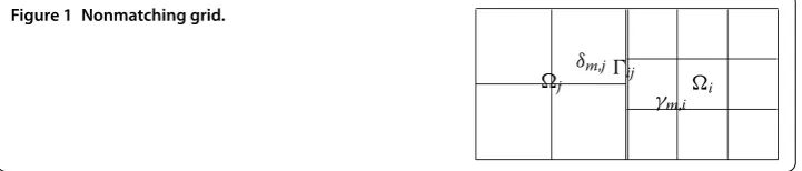
We denoteij the common open edge ofi andj, and let=

ijij. Eachijcan

be regarded as two sides corresponding to the two subdomainsiandj. We define one

of the sides ofijas mortar denoted byγm,iand the other one as nonmortar denoted by

δm,j, heremrepresents the indexing ofij(see Figure ). We assume that: () the mortar for

γm,i=δm,j=ijis chosen by the conditionρjρi; () there is at least one subdomain which

has two mortar sides associated with each cross point; ()hihj,i.e.,hi/hjis bounded. The

first condition used in choosing mortar sides is essential (see the numerical tests in []). The last condition is technical but not essential for the convergence analysis. Along each ij, there are two independent and different -D meshes which are denoted byThi(γm,i) and Tj

h(δm,j). For each nonmortar sideδm,j=ij, we denote byMhj(δm,j)⊂L(ij) an auxiliary

Figure 1 Nonmatching grid.

j i

δm,j_ij

test space whose functions are piecewise constant onT_hj(δm,j). We denote byQm theL

-orthogonal projection from theL₍

ij) space to theMhj(δm,j) space.

Now we define the mortar-type rotatedQspace as follows:

Vh=

v=

N

i=

vi∈Xh() :Qm(vi|γm,i) =Qm(vj|δm,j),∀γm,i=δm,j⊂

, (.)

herevi|γm,iis the restriction ofvi∈Xh(i) to the mortar sideγm,i, andvj|δm,j is the

restric-tion ofvj∈Xh(j) to the nonmortar sideδm,j. The condition in (.) for each interface is

calledmortar condition. The mortar-type rotatedQelement approximation of problem (.) is: finduh∈Vhsuch that

ah(uh,vh) = (f,vh), ∀vh∈Vh, (.)

where

ah(uh,vh) = N

i=

ah,i(uh,vh), ah,i(uh,vh) =

E∈Th(i)

E

ρi∇uh∇vhdx.

It can easily be shown thatah(·,·) is positive definite onVh, which yields the existence

and uniqueness of the discrete solution. The error estimate between the discrete and the continuous solution is discussed in [].

Since the mortar condition depends on both the degrees of freedom on the interfaces and the ones near the interfaces, it is difficult to construct a preconditioner directly for (.). To overcome this difficulty, we introduce a new discrete space and an auxiliary prob-lem which is equivalent to probprob-lem (.).

For each v∈Vh, we define an elementv˜= iN=v˜i∈Xh() that satisfies the following

conditions:

• for anye∈(N_i=ie_,h)∪(_mTi h(γm,i)),



|e|

e ˜

v ds= 

|e|

e

v ds; (.)

• for anyψ∈Mhj_(δ m,j),

δm,j ˜

vψds=

δm,j ¯

vψds, (.)

wherev¯∈L_(γ

m,i)is a piecewise constant function on elements ofT_hi(γm,i)such that ¯

v|e=_|_e|evi|γm,idsfor anye∈T i

h(γm,i). Note that the average value ofv˜one∈Thj(δm,j)

can be calculated by(.).

By the above definition, allv˜associated withvform a spaceV˜h⊂Xh() as

˜

Vh=

˜

v=

N

i=

˜

vi∈Xh() :v∈Vh

.

Lemma .([]) For any pair of v∈Vh,v˜∈ ˜Vhdefined above,the following is true:

ah(v,v)ah(˜v,˜v). (.)

Now we introduce the auxiliary problem, that is, to findu˜∈ ˜Vhwhich satisfies

ah(u˜,˜v) =f(v˜), ∀˜v∈ ˜Vh. (.)

Define an operatorA˜h:V˜h→ ˜Vhby

(A˜hv˜,w˜) =ah(v˜,w˜), ∀˜v,w˜∈ ˜Vh.

From the above lemma, we only need to construct a preconditioner for the operatorA˜h.

3 BDDC algorithm

In this section, we introduce our BDDC preconditioner for problem (.) and describe the BDDC algorithm.

We first define a discrete harmonic operatorHiassociated with the rotatedQelement: for anyv∈Xh(i), letHiv∈Xh(i) such that

ah,i(Hiv,w) = , ∀w∈Xh(i),

 |e|

eHiv ds=

 |e|

ev ds, ∀e∈∂ e i,h,

hereX

h(i) ={v∈Xh(i) :

ev ds= ,∀e∈∂ei,h}. LetXh(∂i) =Hi(Xh(i)). We defineH

as a corresponding piecewise harmonic operator on the auxiliary spaceV˜hbyH|i=Hi.

In order to introduce our domain decomposition method, we decompose the auxiliary discrete spaceV˜has follows:

˜

Vh=XhP()⊕ ˜Vh() and XhP() = N

i=

X_h(i), (.)

where the spaceV˜h() is a piecewise harmonic function space defined as

˜

Vh() =H(V˜h) =

v∈ ˜Vh:v|i=Hi(v|i),i= , , . . . ,N

.

We define a spaceX˜h() ={v∈ Ni=Xh(∂i) :

γm,iv|ids=

δm,jv|jds,∀γm,i=δm,j⊂}.

The spaceX˜h() is betweenV˜h() and Ni=Xh(∂i), and our BDDC preconditioner is

mainly constructed on this space.

As we know, the technical aspect in DDMs is that the preconditioner includes a coarse problem which can enhance the convergence. In view of the characteristic of the space

˜

Xh(), we select the standard coarse spaceVH() which is the rotatedQfinite element space associated with the coarse partition TH(), and it satisfies primal constraints on

subdomain interfaces.

The substructure spaceV˜ (i) with constraints is defined by

˜ V (i) =

v∈Xh(∂i) :

ij

v ds= ,∀ij⊂∂i

DenoteV˜ () = N_i=V˜ (i). The coarse space and the product spaceV˜ () play an

im-portant role in the description and analysis of our iterative method.

To present our BDDC preconditioner, we introduce several space transfer operators. Define an interpolation operatorIH:V˜h→VH() by

ijIHv ds |ij| =

ijv ds

|ij| , ∀ij⊂.

The intergrid transfer operatorIh:VH()→ ˜Xh() is defined by

eIhv ds |e| =

ev ds

|e| , ∀e∈∂

e

i,h(i= , . . . ,N).

Define an extension operatorRT

i :Xh(∂i)→ ˜Vh() as

• for anye∈γm,i⊂∂iT i

h(γm,i), _|_e|

eR T

iv|γm,ids=

 |e|

ev|γm,ids;

• for anye∈_γr,j⊂∂iT_hj(γr,j), _|_e|

eRTiv|γr,jds= ;

• for anye∈_nT_hj(δn,j), _|_e|

eR T

iv|δn,jdssatisfies(.).

Its transposeRi:V˜h()→Xh(∂i) is defined by

(Riw,v) =

w,RT_iv, ∀w∈ ˜Vh(),v∈Xh(∂i).

DenoteRT_i|_V˜ (i):V˜ (i)→ ˜Vh() byR T

,i, the corresponding transposeR ,i:V˜h()→ ˜

V (i) is defined by

(R ,iw,v) =

w,RT _,iv, ∀w∈ ˜Vh(),v∈ ˜V (i).

We also need to define another prolongation operatorEi:Xh(i)→ ˜Vhas follows:

• ife∈e_i,h, then_|e_|eEiv ds=_|_e|

ev ds;

• ife∈T_hi(γm,i),γm,i⊂∂i, then_|_e|

eEiv ds=

 |e|

ev ds;

• ife∈T_hk(γs,k),∀γs,k,k=i, then_|_e|

eEiv ds= ;

• ife∈_sT_hj(δs,j), it follows from(.)that_|_e|

eEiv dscan be obtained by the edge

average values on associated mortar sides; • else,_|_e|eEiv ds= .

In what follows, we describe our BDDC preconditioning algorithm, we apply the ba-sic framework of additive Schwarz method (or parallel subspace correction method []). From the decomposition (.), we only need to choose appropriate subspace solvers.

First of all, the coarse subspace solverBH:VH()→VH() is defined by

(BHuH,vH) =ah(uH,vH), ∀uH,vH∈VH().

On each subdomain, similar operatorsBi:V˜ (i)→ ˜V (i) andBP,i:Xh(i)→Xh(i)

are defined, respectively, by

(Biu,v) =ah,i(u,v), ∀u,v∈ ˜V (i),

Remark . The bilinear form on the coarse space can be different from that on substruc-ture space, here we only use the exact solvers. On each subdomain, we avoid the possible singularity of local subproblem and we need not modify the bilinear forms.

Now we define our BDDC preconditioner as

Bbddc=RTB–HR+

N

i=

RT _,iB–_i R ,i+ N

i= B–_p,i,

whereRT

=

N

i=RTi Ih,Ris the corresponding transpose defined by

(Rw,v) =

w,RT_v, ∀w∈ ˜Vh(),v∈VH().

LetPbe an operator fromV˜h() toVH() defined by

ah(Pu,v) =ah

u,RT_v, ∀u∈ ˜Vh(),v∈VH(),

PiandPp,ibe the operators fromV˜h() toV˜ (i) andXh(i) defined, respectively, by

ah,i(Piu,v) =ah

u,RT _,iv, ∀u∈ ˜Vh,v∈ ˜V (i),

ah(Pp,iu,v) =ah(u,v), ∀u∈ ˜Vh,v∈Xh(i).

Then the BDDC preconditioned operatorPbddc=BbddcA˜hcan be written as

Pbddc=RTP+

N

i=

RT _,iPi+ N

i= Pp,i.

We have the following main result.

Theorem . The BDDC preconditioned operator Pbddcsatisfies

ah(u,u)ah(Pbddcu,u)

 +logH

h



ah(u,u), ∀u∈ ˜Vh,

where H/h=maxi(Hi/hi).

4 Technical tools

In this section we state and prove a few technical lemmas necessary for the proof of The-orem .. Our theoretical analysis is based on the substructuring theory of conforming elements.

We assumeVh₍

i) be the bilinear conforming element space associated with the

par-titionTh(i). We split the interface∂iinto four open edgesE, and define a restriction

operatorI_E:Vh_(∂

i)→Vh(∂i) (Vh(∂i) =Vh(i)|∂i) as: for anyv∈Vh(∂i)

I_Ev=

v, onE, , on∂i\E.

Lemma .([]) For an edgeEof∂i,then for any v∈Vh(∂i),we have

I_Ev_H/_(∂

i)

 +logHi

hi

vH/_(∂

i).

Remark . The above lemma is related to vertex-edge-face arguments in substructuring methods, in view of the characteristic for the rotatedQ element, here the results only concern the inequalities for faces.

LetVh/₍

i) be the conforming element space of bilinear continuous functions on the

partitionTh/(i) which is constructed by joining the midpoints of the edges of elements

ofTh(i). We now introduce a local equivalence mapMi:Xh(i)→Vh/(i) as follows

(cf.[]).

Definition . Givenv∈Xh(i), we defineMiv∈Vh/(i) by the values ofMivat the

vertices of the partitionTh/(i).

• IfPis a central point ofE,E∈Th(i), then

(Miv)(P) =

 

ei∈∂E



|ei|

ei

v ds.

• IfPis a midpoint of one edgee∈∂E,E∈Th(i), then

(Miv)(P) =



|e|

e

v ds.

• IfP∈i,h\∂i,h, then

(Miv)(P) =

 

ei



|ei|

ei

v ds,

where the sum is taken over all edgeseiwith the common vertexP,ei∈∂Ei,

Ei∈Th(i).

• IfP∈∂i,h, then

(Miv)(P) = |

el|

|el|+|er|



|el|

el

v ds

+ |er|

|el|+|er|



|er|

er

v ds

,

whereel∈∂E∩∂iander∈∂E∩∂iare the left and right neighbor edges ofP,

E,E∈Th(i). IfPis a vertex ofi, thenE=E.

Define the pseudo-inverse mapM+

i :Vh/(i)→Xh(i) by



|e|

e

M+

iv ds=v(P), ∀v∈Vh/(i),

wheree∈∂E,E∈Th(i),Pis the midpoint ofe. Obviously, we have

M+

For the operatorsMiandM+i, we have the following results (see []):

|Miv|H₍

i) |v|H_h(i), ∀v∈Xh(i); _M+

ivH_h(i) |v|Hh(i), ∀v∈V h/₍

i).

(.)

Lemma . For any ui∈ ˜V (i),we can split uiinto ui=

ij⊂∂iuij,and we have

|uij|_H

h(i)

 +log(Hi/hi)

|ui|_H

h(i), (.)

where uij∈ ˜V (i), and for any e∈eij,

euijds/|e|=

euids/|e|; for any e∈∂ei,h \ij,

euijds/|e|= .

Proof By (.), Lemma ., the inverse trace theorem, the trace theorem, and the Poincaré inequality, we obtain

|uij|_H

h(i)≤M

+

iHiI_E(Miuij)_∂ iHh(i) HiI_E(Miuij)_∂

iHh(i) I_E(Miuij)_∂

iH/(∂i)  +log(Hi/hi)

MiuiH/_(∂

i) ≤ +log(Hi/hi)

MiuiH₍

i)  +log(Hi/hi)

|Miui|H₍

i)  +log(Hi/hi)

|ui|_H

h(i),

whereHiis a piecewise bilinear conforming element harmonic operator, and we have used

the minimal energy property of discrete harmonic functions.

5 Proof of Theorem 3.1

In the proof of Theorem . we use the abstract framework of ASM methods (see []), we need to prove three assumptions. Assumption II follows from the standard coloring argument, we only need to prove Assumption I and Assumption III.

First we show the following stability of the decomposition.

Lemma .(Assumption I) For any u∈ ˜Vh,we have the following decomposition:

u=RT_uH+ N

i=

RT _,iui+ N

i=

up,i, uH∈VH(),ui∈ ˜V (i),up,i∈Xh(i), (.)

which satisfies

ah(uH,uH) + N

i=

ah,i(ui,ui) + N

i=

ah,i(up,i,up,i)ah(u,u). (.)

Proof First we show the decomposition (.). For any functionu∈ ˜Vh, letup,i=Pp,iuand

uH=IHu, obviouslyu–

N

denoteu =u–N_i=up,i–IhuH,ui=u |i. From the definition ofIHandIh, we have

ij

uids=

ij

u ds=

ij

(u–IhuH)ds=

ij

(u–uH)ds= ,

and by the definition ofRT

,i, we get

RT_uH+ N

i=

RT _,iui+ N

i= up,i=

N

i=

RT_iIhuH+ N

i= RT_i

u–

N

i=

up,i–IhuH

+

N

i= up,i

=

N

i= RT_i

u–

N

i= up,i

+

N

i= up,i

=u–

N

i= up,i+

N

i= up,i

=u,

where we have used the factN_i=RT_iu=u,∀u∈ ˜Vh(). Henceui∈ ˜V (i) and the equality

(.) holds.

Now we prove the stability of decomposition (.). Let u¯ij =

iju ds/|ij|. Using

Lemma . in [], Poincaré-Friedrichs’ inequality and scaling argument, we derive

ij,ik⊂∂i

|¯uij–u¯ik|

 ₌

ij,ik⊂∂i



|ij|

ij

(u–u¯ik) 

ik⊂∂i



H_iu–u¯ik



L₍

i)+|u|



H

h(i)

|u|_H

h(i). (.)

From (.) and the discrete equivalent norm, we have

ah(uH,uH) = N

i=

ah,i(uH,uH) N

i= ρi

ij,ik⊂∂i

|¯uij–u¯ik|

_a

h(u,u). (.)

SincePp,iis an orthogonal projection with respect toah,i(·,·), we obtain

N

i=

ah,i(up,i,up,i) = N

i=

ah,i(Pp,iu,Pp,iu)≤ah(u,u). (.)

Meanwhile, from the fact that the harmonic function has minimal energy norm and (.)-(.), we deduce

N

i=

ah,i(ui,ui) =ah(u ,u )

=ah

u–

N

i=

up,i–IhuH,u– N

i=

ah(u,u) + N

i=

ah,i(up,i,up,i) +ah(IhuH,IhuH) (.)

ah(u,u). (.)

So (.)-(.) lead to (.).

Next we state the local stability as follows.

Lemma .(Assumption III) For any u∈ ˜V (i),we have

ah

RT _,iu,RT _,iu

 +logH

h



ah,i(u,u). (.)

For any uH∈VH(),we have

ah

RT_uH,RTuH

 +logH

h



ah(uH,uH). (.)

Proof To prove (.) we first introduce a functionθm= Ni=θm,i∈ ˜Vh associated with a

mortar sideγm,i⊂, which satisfies the following:

• for anye∈Ti h(γm,i),

 |e|

eθm,i|γm,ids= ;

• for anye∈_r=mTi h(γr,i),

 |e|

eθm,i|γr,ids= ;

• for anye∈_nT_hj(δn,j), _|_e|

eθm,j|δn,jdssatisfies(.).

Then we can decomposeRT _,iu∈ ˜Vh() as follows:

RT _,iu=RT_iu=H

γm,i⊂∂i

Ih

θm,i(Eiu)

= γm,i⊂∂i

HIh

θm,i(Eiu)

, (.)

here we have used the fact that the degrees of freedom on the interfaceof the functionu are as same as that of_γ

m,i⊂∂iIh(θm,i(Eiu)), and the operatorIhis defined by the average

values on the edge elements,i.e.,



|e|

e

Ih

θm,i(Eiu)

= 

|e|

e

θm,ids·



|e|

e

Eiu ds, ∀e∈∂eh,i.

Note that the support ofH(Ih(θm,i(Eiu))) is on¯i∪ ¯j, and using Lemma . in [] we

have

ah

HIh

θm,i(Eiu)

,HIh

θm,i(Eiu)

ρiHIh

θm,i(Eiu)



H

h(i). (.)

Since the degrees of freedom on the interface∂iofHi(Ih(θm,i(Eiu))) are only nonzero on

the edgeγm,i, using Lemma ., we deduce _HIh

θm,i(Eiu)_H

h(i) =Hi

Ih

θm,i(Eiu)_H

h(i)

 +log(Hi/hi) 

|Hiu|_H

h(i)

 +log(Hi/hi) 

|u|_H

h(i). (.)

Using similar techniques to those in (.), and summing over all subdomains, we can complete the proof of (.).

6 Numerical results

In this section, we show numerical results of our method using the model problem

–div(ρ∇u) =f, in, u= , on∂,

where= [, ]_{. The domain is composed ofM×Msub-squares, their mesh sizes are} H, and the sub-squares are divided into smaller ones with mesh sizeshmin mortar

subdo-mains; andhnin nonmortar subdomains. The coefficientρis either  or k(k= , , ).

We use the preconditioned conjugate gradient (PCG) method with zero initial guess for the discrete system of equations. The stopping criterion for the PCG method is when the -norm of the residual is reduced by the factor of – _{of the initial guess. An estimate} for the condition number of the corresponding system is computed by using the Lanczos algorithm.

In Table , we show the number of iterations and the condition numbers with different ratioH/hn. In Figure , we plot the condition number as the function ( +log(H/h))for

Table 1 The number of iterations and condition numbers forh_m/h_n= 2/3

M×M H/hn= 4 H/hn= 16

k= 2 k= 4 k= 6 k= 2 k= 4 k= 6

4×4 10 (3.30) 10 (3.30) 10 (3.30) 12 (5.15) 12 (5.15) 12 (5.15) 8×8 11 (3.30) 11 (3.34) 11 (3.32) 12 (5.30) 13 (5.34) 13 (5.34) 16×16 11 (3.24) 12 (3.21) 13 (3.21) 13 (5.32) 13 (5.39) 14 (5.39) 32×32 11 (3.24) 12 (3.24) 12 (3.24) 15 (5.37) 15 (5.41) 15 (5.41)

 domains. From the results in Table  and Figure , we see that the convergence of our method is quasi-optimal since the number of iterations is independent of the jumps of the coefficients, and almost independent of the mesh size.

Competing interests

The authors declare that they have no competing interests.

Authors’ contributions

All results belong to YJ and JC. All authors read and approved the final manuscript.

Acknowledgements

The work was supported by the National Natural Science Foundation of China (Grant Nos. 11371199 and 11301275), Jiangsu Provincial 2011 Program (Collaborative Innovation Center of Climate Change), the Program of Natural Science Research of Jiangsu Higher Education Institutions of China (Grant No. 12KJB110013), the Doctoral fund of Ministry of Education of China (Grant No. 20123207120001), and Jiangsu Key Lab for NSLSCS (Grant No. 201306). Moreover the authors are grateful to anonymous referees for their constructive comments and suggestions.

Received: 14 January 2014 Accepted: 17 March 2014 Published:03 Apr 2014

References

1. Dohrmann, C: A preconditioner for substructuring based on constrained energy minimization. SIAM J. Sci. Comput.

25, 246-258 (2003)

2. Mandel, J, Dohrmann, C: Convergence of a balancing domain decomposition by constraints and energy minimization. Numer. Linear Algebra Appl.10, 639-659 (2003)

3. Li, J, Widlund, O: FETI-DP, BDDC, and block Cholesky methods. Int. J. Numer. Methods Eng.66, 250-271 (2006) 4. Mandel, J, Dohrmann, C, Tezaur, R: An algebraic theory for primal and dual substructuring methods by constraints.

Appl. Numer. Math.54, 167-193 (2005)

5. Kim, H: A BDDC algorithm for mortar discretization of elasticity problems. SIAM J. Numer. Anal.46, 2090-2111 (2008) 6. Kim, H: A FETI-DP formulation of three dimensional elasticity problems with mortar discretization. SIAM J. Numer.

Anal.46, 2090-2111 (2008)

7. Kim, H, Lee, C, Park, E: A FETI-DP formulation for the Stokes problem without primal pressure component. SIAM J. Numer. Anal.47, 4142-4162 (2010)

8. Le Tallec, P, Mandel, J, Vidrascu, M: A Neumann-Neumann domain decomposition algorithm for solving plate and shell problems. SIAM J. Numer. Anal.35, 836-867 (1998)

9. Rannacher, R, Turek, S: Simple nonconforming quadrilateral Stokes element. Numer. Methods Partial Differ. Equ.8, 97-111 (1992)

10. Bernardi, C, Maday, Y, Patera, A: Domain decomposition by the mortar element method. In: Kaper, HG, Garbey, M, Pieper, GW (eds.) Asymptotic and Numerical Methods for Partial Differential Equations with Critical Parameters, pp. 269-286. Kluwer Academic, Dordrecht (1993)

11. Marcinkowski, L: Additive Schwarz method for mortar discretization of elliptic problems withP1nonconforming elements. BIT Numer. Math.45, 375-394 (2005)

12. Wang, F, Chen, J, Xu, W, Li, Z: An additive Schwarz preconditioner for the mortar-type rotatedQ1FEM for elliptic problems with discontinuous coefficients. Appl. Numer. Math.59, 1657-1667 (2009)

13. Chen, J, Xu, X: The mortar element methods for rotatedQ1element. J. Comput. Math.20, 313-324 (2002) 14. Xu, J: Iterative methods by space decomposition and subspace correction. SIAM Rev.34, 581-613 (1992) 15. Xu, J, Zou, J: Some nonoverlapping domain decomposition method. SIAM Rev.40, 857-914 (1998) 16. Toselli, A, Widlund, O: Domain Decomposition Methods: Algorithms and Theory. Springer, Berlin (2005)

10.1186/1687-2770-2014-79

Cite this article as:Jiang and Chen:A BDDC algorithm for the mortar-type rotatedQ1FEM for elliptic problems with