Solving Multi-Mode Time-Cost-Quality Trade-off Problem in Uncertainty Condition Using a Novel Genetic Algorithm

http://www.sciencepublishinggroup.com/j/ijmfs doi: 10.11648/j.ijmfs.20170303.11

Solving Multi-Mode Time-Cost-Quality Trade-off Problem in

Uncertainty Condition Using a Novel Genetic Algorithm

Hasan Hosseini-Nasab

1, *

, Masour Pourkheradmand

1

, Naser Shahsavaripour

2

1

Industrial Engineering Department, Yazd University, Yazd, Iran

2

Department of Industrial Management, Vali-e-Asr University, Rafsanjan, Iran

Email address:

[email protected] (H. Hosseini-Nasab), [email protected] (M. Pourkheradmand), [email protected] (N. Shahsavaripour)

*

Corresponding author

To cite this article:

Hasan Hosseini-Nasab, Masour Pourkheradmand, Naser Shahsavaripour. Solving Multi-Mode Time-Cost-Quality Trade-off Problem in Uncertainty Condition Using a Novel Genetic Algorithm. International Journal of Management and Fuzzy Systems.

Vol. 3, No. 3, 2017, pp. 32-40. doi: 10.11648/j.ijmfs.20170303.11

Received: May 13, 2017; Accepted: June 14, 2017; Published: July 21, 2017

Abstract:

In this paper a Fuzzy Discrete Time-Cost-Quality Trade-off Problem (FDTCQTP), is presented. All of three main factors of a project are considered in uncertainty condition using fuzzy theory. Time, cost and quality are considered as fuzzy trapezoidal numbers and a novel Genetic Algorithm; Super Genetic Algorithm (SGA) is introduced to solve the problem. Project network paths are calculated via a new algorithm which it can be very useful for complex project networks and in order to comparing the fuzzy numbers, a new Fuzzy Number Ranking (FNR) method is introduced. The proposed algorithm is compared with classic GA by ANOVA, and the results demonstrate its efficiency. An applied example is used to more details.

Keywords:

Project Scheduling, Time-Cost-Quality Trade-off Problem, Metaheuristics, Genetic Algorithm, Fuzzy Theory, Fuzzy Number Ranking, CPM, ANOVA

1. Introduction

According to American national standard institute, project management is: “The application of knowledge, skills, tools and techniques to project activities to meet project requirements” [1]. In project management, it is sometimes required to complete the project before the normal due time .Naturally, in such cases; the duration of performing some of the activities must be decreased. Decreasing the time leads to increasing resources consuming, and costs.

Since resources, execution methods and technology types in real world projects are represented by discrete values, for real world applications Discrete Time-Cost Trade-off Problem (DTCTP) is applied [2] The DTCTP is known as an NP-hard problem [3], and no exact solution method can be found to have the required efficiency for solving DTCTP. However, there are some approaches based on heuristic algorithms for solving DTCTP [4, 5]. Quality is another important factor in executing the project which requires considerable attention. Clearly, reduction in time or changing execution methods lead to changes in quality of project

execution. So a DTCTP can be generalized to a Discrete Time-Cost-Quality trade-off problem (DTCQTP).

A project consists of different parts of an activity. These activities have different execution modes in which each mode has its own time-cost-quality execution.

Babu and Suresh were the first who suggested that the quality of a completed project may be affected by project crashing [6]. El-Rayes and Kandil [7], presented a model that is designed to transform the traditional two-dimensional time-cost trade off analysis to an advanced three-dimensional time-cost-quality trade-off analysis. Iranmanesh and Skandari [9], found Pareto- optimal front of time, cost and quality of a project, whose activities could be done in different discrete modes and each mode has a different cost, time and quality. They proposed Fast PGA algorithm that was meta-heuristic and was developed based on a version of GA.

Modarres et al [2], used fuzzy theory to manage the uncertainty of quality, and considered the two other factors as crisp. They also used a novel genetic algorithm to solve the problem. Zhang and Xing [8], presented a fuzzy-multi objective particle swarm optimization to solve the problem, which time, cost and quality described by fuzzy numbers. SantoshMungle and LyesBenyoucef proposed a fuzzy clustering-based genetic algorithm (FCGA) approach, and provided a case study of highway construction to demonstrate the applicability of the proposed approach.

In this study, time-cost and quality of project network activities determined by some experts through fuzzy theory and linguistic variables. These quantities are presented as fuzzy trapezoidal numbers. The aim of a Fuzzy Discrete Time-Cost-Quality Trade-off Problem (FDTCQTP) is to select a set of activities for crashing and an appropriate execution method for each activity such that the cost and time of the project is minimized while the project quality is maximized. In this paper, a novel Genetic Algorithm; Super Genetic Algorithm (SGA) is introduced to solve the problem. A new algorithm is proposed to calculating the project network paths which is very useful for complex project networks, and a new method is introduced to ranking fuzzy numbers. This paper is organized as follows: In section 2, the problem definition and formulation is provided. Section 3, discusses about solution procedure. In section 4, an experimental example is provided. Finally, section 5, concludes the paper.

2. Problem Definition and Formulation

The overall completion time, cost and quality of a construction project are determined by the duration, cost and quality for each activity involved in the project [8]. Activities are demonstrated by arcs in the project network. In order to performing the activities, several modes are available. For example, to performing the activity i, there are several methods and different technologies (modes) which each mode has its own duration, cost and quality. Also, in some cases, resources are not sufficient or technical knowledge is inadequate. In this way, subcontracting should be implemented. Considering that subcontractors perform the activities with different times, costs and qualities, a mathematical modeling is required to achieve the optimum solution. The aim of this study is minimizing the time and cost and maximizing the quality of the project.

Notations of the problem are as follows: Parameters:

Mij Set of available execution modes for activities i and j,

where (i, j)∈E

Cɶ_ijk Fuzzy direct cost of activities i and j performed by

execution mode k;

Tɶ_ijk Fuzzy duration of activities i and j performed by

execution mode k;

qɶ_ijk Fuzzy quality of activities i and j performed by

execution mode k;

ij

w Quality weight of activities i and j in the project,

Decision variables:

ijk

y 1 if mode k is assigned toactivities i and j

0 otherwise

  

i

xɶ Early event time i, (i={1,2,...,m}) The model of FDTCQTP is as follow:

. .

IJ ij ijk ijk

ij E k M

Max Q w q y

∈ ∈

 

= 



∑ ∑



ɶ _{ɶ (1)}

C .

IJ ijk ijk

ij E k M

Min C y

∈ ∈

 

= 



∑ ∑



ɶ ɶ ₍₂₎

1

T _n

Min ɶ =xɶ −xɶ (3)

1 ij

ijk

k M∈ y =

∑

, ij∈E (4)

1

ij ij E∈ w =

∑

(5)

0

i

x ≥ _, i V∈ ₍₆₎

{ }

0,1

ijk

y ∈ , ij∈E k, ∈Mij (7)

Equation (1) maximizes the total project quality and Equations. (2), (3), minimize the total project cost and time respectively. Equation (4), guarantees that one and only one execution mode is assigned to each activity. In Equation (5) summation of activities’ important weight factor should be equal to 1.

3. Solution Procedure

To solve the problem it is necessary to calculate the time, cost and quality of the project.

To calculating the duration of performing the project, critical path method (CPM) is used. To calculating the CPM, it is first necessary that the project network paths be identified.

3.1. Calculating the Project Network Paths

In this paper, to calculate different paths of a project network, a new algorithm is presented.

Let m be the number of nodes and A_{m m×} =_a_ij_ be the node-node adjacency matrix with the following notations,

1 if node i starts arc j

0 otherwise ij a =           (8)

Figure 1. Flowchart of detecting the network project paths.

After detecting the paths, fuzzy time of the existing activities in these paths are added up and the biggest fuzzy number is identified using FNR algorithm.

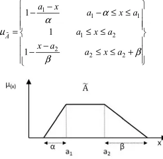
3.2. Fuzzy Number Ranking Method

FNR method is described using the following algorithm. The fuzzy number of Aɶ is set in [0, 1] by µ (x)_Aɶ membership function (Figure 2). The trapezoidal fuzzy number of Aɶ is shown as Aɶ=

(

a a a1, 2, A,

β

A

)

which its

membership function is defined by:

1

1 1

1 2

2

2 2

1

1

1

A

a x

a x a

a x a

x a

a x a

α α

µ

β β

 ₋ 

− − ≤ ≤

 

 

 

= ≤ ≤ 

 ₋ 

 _{− ≤ ≤ +} 

 _



ɶ (9)

Figure 2. Definition of Aɶ=

(

a a1, 2,aA,βA

)

.

Suppose that and

B

~

=

(

b

₁

,

b

₂

,

a

_B

,

β

_B

)

are two fuzzy numbers, whose summation and multiplying is computed by:

(

a b a b aA aB A B

)

B

A~+ ~= ₁ + ₁, ₂ + ₂, + ,

β

+

β

(10)

(

a b a b aA B aB A

)

B

A~−~= ₁− ₂, ₂− ₁, +

β

, +

β

(11)

If _K≻0; K

() (

.A~= Ka₁,Ka₂,Ka_A,K

β

_A

)

(12)

If _{K ≺0}; K

() (

.A~= Ka₂,Ka₁,−K

β

_A,−Ka_A

)

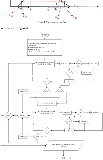
(13)

To comparing the fuzzy numbers

A

ɶ

_and

B

ɶ

_,

x

_2A,

x

_2B are calculated for different values of Y, and at each iteration, a pre-defined superiority is attributed to the bigger number. The superiority becomes more when y getting close to 1.

Y=1/ƞ (14)

Ƞ is an arbitrary number which determines the number of intervals in [0, 1]. For example if Ƞ=10, then y, at each iteration, has values of 0, 0.1, 0.2, …, 0.9, 1.

2A

x

,

x

_2B are calculated as follows: For the fuzzy number

A

ɶ

:

(

)

2A 2

1 y β

A

1A 1

(y 1)

A

x

= + −

a

α

(16)

for the fuzzy number

B

ɶ

:

(

)

2B 2

1 y β

B

x

= + −

b

(17)

1B 1

(y 1)

B

x

= + −

b

α

(18)

Finally the number with the higher superiority is the bigger one. (Figure 3). In case of equality these steps will repeat for

1A

x

,

x

_1B.

Figure 3. Fuzzy ranking method.

The FNR algorithm is shown in Figure 4.

3.3. Introducing a Novel GA; Super GA

As it mentioned in part 1, FDTCQTP is known as NP-hard problem. So it is required to use a heuristic or metaheuiristic algorithm to solve it. In this paper SGA is presented which it has higher performance with respect the classic GA. It is explored using ANOVA in section (5).

In classic GA, selection probability of chromosomes represents by;

( )

( )

( )

∑ = _N i f i f i P 1 (19)

Which f(i) denotes the fitness value of chromosome(i) in current generation. It can be say that this fitness value is not enough strong to be cause of a good chromosome to be selected. Also direct selection methods can be used, but some other defects still exist. In direct selection methods, there is no chance for a bad chromosome which has a great potential to become a very good chromosome using partial disturbance. So, the new fitness value, fnew is introduce as

follow:

( )

( )

        ₋ = σ µ i f e i new

f (20)

fnew is the new fitness function, and µ and σ, are the mean

and standard deviation of the all fitness functions at the same iteration. See table 1 for more details.

( )

( )

( )

∑ = _N i new f i new f i P 1 (21)

Equation (21), calculates the new selection probability of each chromosome. The selection probability of chromosome (5) is equal to 0.24 (f(5) =0.24), which it has not distinct

different with chromosomes (4) (f(4) =0.22). However, using

the new fitness value, selection probability of chromosome (5) increased to 0.52 while the other fitness values are not zero and they can be selected with the lower probability. Using this technique, a chromosome, with the small superiority, has a good chance to be selected. This change improved classic GA so as it can be say it is better to use SGA instead of classic GA, always.

Table 1. Comparing of new and classic fitness functions.

No. Fitness function value classic Selection probability (f-µ)/σ e(f-µ)/σ New Selection probability

1 3.5 0.155556 -1.41421 0.243117 0.030862 2 4 0.177778 -0.70711 0.493069 0.062592

3 4.5 0.2 0 1 0.126944

4 5 0.222222 0.707107 2.028115 0.257457 5 5.5 0.244444 1.414214 4.11325 0.522152 sum 22.5

µ 4.5 σ2 _0.5

3.4. Proposed Algorithm Implementation

In order to solve the problem using the presented algorithm, it is necessary first to define the chromosome.

Each chromosome has n genes which n is the number of project network activities. Each gene contains a random number between 1 and maximum execution modes for each activity (Mij). For example, the following chromosome shows

that activity 1 will execute with mode ith, activity 2 with mode jth and…activity n with mode kth. (Figure 5).

Figure 5. Chromosome of the problem. i, j, k € (1, maximum number of available modes of each activity).

3.5. Calculating Fitness Function

To calculate fitness function for each chromosome three parameters of time, cost and quality should be calculated.

For each chromosome, time, cost and the quality of project should be calculated.

( )

i

C~ ; is theTotal cost of project.

( )

i

T~ ; is thetotal project time of project which is calculated by CPM method.

( )

i

Q~ ; is the quality of project which is obtained by Equation 20.

( )

i =

∑

nw_i q_ij Q 1 ~ . ~ (22)

The fitness function (F(i)) of chromosome “i” is calculated

by following equation:

( )

( )

( )

( )

γ

γ

γ

γ

γ

γ

+ − + − + + − + − + + − + − = min max max min max min min max min ~ ~ ~ ~ . ~ ~ ~ ~ . ~ ~ ~ ~ . Q Q i Q Q w C C C i C w T T T i T w i

F _{t c q} (23)

Where, wc, wt and wq are the planner-specified weight.

They indicate the relative importance of project cost,

duration and quality respectively. And wt+ wc+ wq=1.0.

max ~

maximal and minimal values of cost, duration and quality in the current population respectively. γ is a very small positive number in order to prevent dividing by zero in the fitness function.

In this paper, two -point crossover and uniform crossover of Hasançebi and Erbatur [10] with pre -specified weights are used. Also two-point mutation is used. Two random chromosomes are selected to show the operators.

Parent 1= [2,1,5,3,2,4,1,5,3,6,1,7] Parent 2= [4,3,2,5,4,1,3,2,5,2,4,6]

Applying the operators, the offspring produced from the parents are as follows:

Two-cut-point crossover with random points (e1=4, e2=7).

Offspring 1= [2,1,5,5,4,1,3,5,3,6,1,7] Offspring 2= [4,3,2,3,2,4,1,2,5, 2,4,6]

Uniform crossover with a random mask chromosome [1,1,0,1,0,0,1,0,0,1,1,0].

Offspring 1= [4,3,5,5,2,4,3,5,3,2,4,7] Offspring 2= [2,1,2,3,4,1,1,2,5,6,1,6]

Two point mutation with random points (e1=6, e2=12).

Offspring 1= [2,1,5,3,2,7,1,5,3,6,1,1]

The steps of our proposed SGA are summarized in Figure 6.

Figure 6. Flowchart of proposed algorithm.

4. Numerical Example

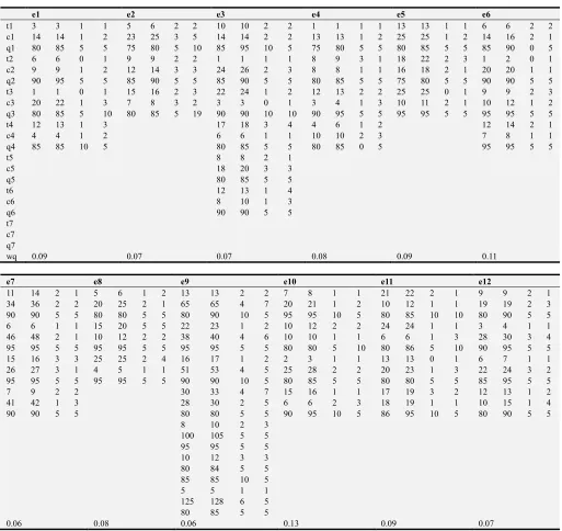
To show the efficiency of the suggested algorithm, an example is presented here. This example deals with a project network (Figure 7). This project network consists of 12 activities. There are several modes for executing each activity. Each mode has its own time, cost and quality that are shown in terms of trapezoidal numbers in table 2. The effect of weight of each activity in total quality (we) is also

considered in Table 2.

Table2. Activities executions modes.

e1 e2 e3 e4 e5 e6

t1 3 3 1 1 5 6 2 2 10 10 2 2 1 1 1 1 13 13 1 1 6 6 2 2 c1 14 14 1 2 23 25 3 5 14 14 2 2 13 13 1 2 25 25 1 2 14 16 2 1 q1 80 85 5 5 75 80 5 10 85 95 10 5 75 80 5 5 80 85 5 5 85 90 0 5 t2 6 6 0 1 9 9 2 2 1 1 1 1 8 9 3 1 18 22 2 3 1 2 0 1 c2 9 9 1 2 12 14 3 3 24 26 2 3 8 8 1 1 16 18 2 1 20 20 1 1 q2 90 95 5 5 85 90 5 5 85 90 5 5 80 85 5 5 75 80 5 5 90 90 5 5 t3 1 1 0 1 15 16 2 3 22 24 1 2 12 13 2 2 25 25 0 1 9 9 2 3 c3 20 22 1 3 7 8 3 2 3 3 0 1 3 4 1 3 10 11 2 1 10 12 1 2 q3 80 85 5 10 80 85 5 19 90 90 10 10 90 95 5 5 95 95 5 5 95 95 5 5 t4 12 13 1 3 17 18 3 4 4 6 1 2 12 14 2 1 c4 4 4 1 2 6 6 1 1 10 10 2 3 7 8 1 1 q4 85 85 10 5 80 85 5 5 80 85 0 5 95 95 5 5

t5 8 8 2 1

c5 18 20 3 3

q5 80 85 5 5

t6 12 13 1 4

c6 8 10 1 3

q6 90 90 5 5

t7 c7 q7

wq 0.09 0.07 0.07 0.08 0.09 0.11

e7 e8 e9 e10 e11 e12

11 14 2 1 5 6 1 2 13 13 2 2 7 8 1 1 21 22 2 1 9 9 2 1 34 36 2 2 20 25 2 1 65 65 4 7 20 21 1 2 10 12 1 1 19 19 2 3 90 90 5 5 80 80 5 5 80 90 10 5 95 95 10 5 80 85 10 10 80 90 5 5 6 6 1 1 15 20 5 5 22 23 1 2 10 12 2 2 24 24 1 1 3 4 1 1 46 48 2 1 10 12 2 2 38 40 4 6 10 10 1 1 6 6 1 3 28 30 3 4 95 95 5 5 95 95 5 5 95 95 5 5 80 80 5 10 80 86 5 10 90 95 5 5 15 16 3 3 25 25 2 4 16 17 1 2 2 3 1 1 13 13 0 1 6 7 1 1 26 27 3 1 4 5 1 1 51 53 4 5 25 28 2 2 20 23 1 3 22 24 3 2 95 95 5 5 95 95 5 5 90 90 10 5 80 85 5 5 80 80 5 5 85 95 5 5 7 9 2 2 30 33 4 7 15 16 1 1 17 19 3 2 12 13 1 2 41 42 1 3 28 30 2 5 6 6 2 3 18 19 1 1 10 15 1 4 90 90 5 5 80 80 5 5 90 95 10 5 86 95 10 5 80 90 5 5

8 10 2 3 100 105 5 5 95 95 5 5 10 12 3 3 80 84 5 5 85 85 10 5 5 5 1 1 125 128 6 5 80 85 5 5

0.06 0.08 0.06 0.13 0.09 0.07

The model is programmed in Microsoft Excel using Visual Basic Application (VBA) .In this model the initial chromosomes includes 12 genes in which each gene shows the number related to a random execution mode. In order to calculate fitness function for each chromosome, computing time, cost and quality of that chromosome is required. To find the time of each chromosome, all the available paths in the project network are identified and time of the activities on that path are added up. Then these numbers that are in form of trapezoidal fuzzy numbers are compared with each other through FNR algorithm. The longest time shows critical path of that chromosome. Following network matrix was used to find the network paths (Table 3.).

Table 3. Network matrix was used to find the network paths.

1 2 3 4 5 6 7 8 9

1 0 1 1 0 0 0 0 0 0 2 0 0 0 1 1 0 0 0 0 3 0 0 0 1 0 1 0 0 0 4 0 0 0 0 0 1 1 0 0 5 0 0 0 0 0 0 0 0 1 6 0 0 0 0 0 0 0 1 0 7 0 0 0 0 0 0 0 1 0 8 0 0 0 0 0 0 0 0 1

In this example, there are 18,500,000 solutions. To obtain the optimal solution, the proposed model was used. To solve this model the parameters of the problem are as follows:

size=100, generation number=500, betta=8, alfa=4, two point cross over rate=0.5, uniform cross over rate=0.3, mutation rate=0.2.

These algorithms are coded and implemented in Excel 2007 by the VBA and are run on a PC with CPU Core i7, 2.0 GHz and 4 GB of RAM memory which chromosome

[4,1,3,2,3,4,3,2,4,4,2,4] and its corresponding time, cost and quality, T=[94,104,11,18], C=[127,140,19,26], Q=[90,93,5,4] are obtained as output. Different execution modes of each activity associated with its time, cost and quality are presented in table 4.

Table 4. Final outputs of the NHGAIII.

Wt Wc Wq time Cost Quality Solution chromosome

0.5 0.3 0.2 86 94 8 13 132 146 21 29 90 93 5 3 4 1 3 1 3 4 3 2 2 4 2 4 0.5 0.2 0.3 69 76 7 10 158 171 23 28 91 94 5 4 3 1 3 1 3 4 3 2 2 4 2 3 0.4 0.3 0.3 75 2 7 11 151 166 21 28 91 94 5 4 3 1 3 2 3 4 3 2 2 4 2 4 0.3 0.3 0.4 83 90 9 12 141 157 23 30 90 93 6 3 4 1 6 1 3 4 3 2 2 4 2 1 0.3 0.5 0.2 94 104 11 18 122 136 19 28 89 93 5 3 4 1 3 1 3 4 3 2 4 4 2 4 0.2 0.3 0.5 77 86 10 15 156 169 21 26 92 94 5 4 3 1 3 2 3 3 3 2 4 4 2 3 0.2 0.4 0.4 98 103 8 16 136 146 20 24 90 94 6 4 4 1 3 1 3 3 3 3 4 4 2 4 0.2 0.5 0.3 104 109 8 17 116 129 18 27 88 93 5 3 4 1 3 1 3 4 3 3 4 4 2 4

5. Experimental Evaluation

This section evaluates the performance of SGA and the classical GA. The Weighted Relative Deviation (WRD) is used as a common performance measure to compare these algorithms that are computed by:

min max

min lg

min max

min lg

min max

min lg

~

~

~

~

.

~

~

~

~

.

~

~

~

~

.

Q

Q

Q

Q

w

C

C

C

C

w

T

T

T

T

w

WRD

_t a _c a _q a

−

−

+

−

−

+

−

−

=

Where,

T

~

_alg,

C

~

_alg and Qɶalg are the total project cost

and time and quality for a given algorithm, respectively.

Q

~

_max ,

Q

~

_min,

C

~

_max,

C

~

_min ,

T

~

_max and

T

~

_min are calculated among

final answers of each time the program is run.

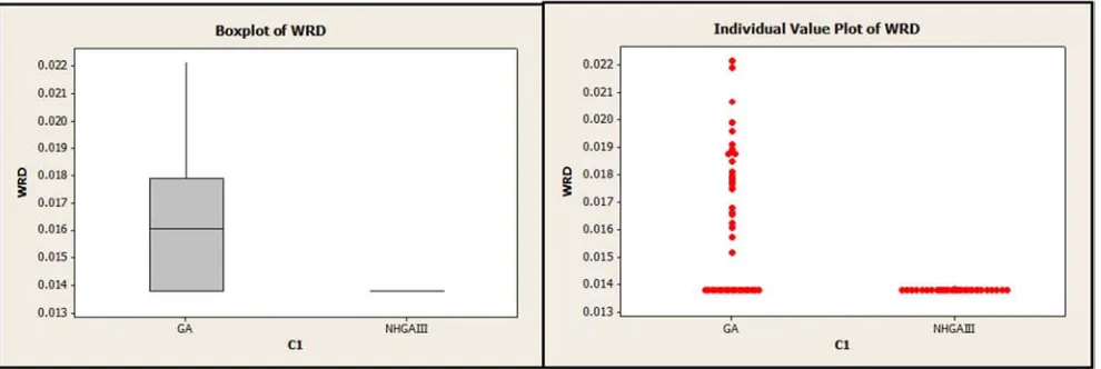
The proposed algorithm, SGA and classic GA are implemented with same parameters for fifty times. Their results are analyzed via the analysis of variance (ANOVA) method. Main hypotheses, containing normality, homogeneity of variance and independence of residuals, are checked and found no bias for questioning the validity of the experiment. The means plot and least significant different (LSD) interval for the SGA and classic GA are shown in Figure 8. It demonstrates that the SGA gives very better outputs than classic GA statistically.

Figure 8. Means plot and LSD intervals for the Super GA and classic GA.

6. Conclusion

This study investigated multi-mode time-cost-quality trade-off problem in uncertainty condition. Due to the big solving space of the algorithm, a new metaheuristics algorithm, Super Genetic Algorithm (SGA), was presented. The efficiency of this algorithm with respect to classic GA was performed by ANOVA. In order to calculate critical path

considering the budget, resources and time constraints and achieving a necessary quality of project in uncertainty condition is suggested.

References

[1] Institute, P. M. (2004). A Guide to the Project Management Body of Knowledge, Third Edition (PMBOK Guides), PMI Publisher.

[2] N.S. Pour, M. Modarres, R. T. Moghaddam (2012). "Time-Cost-Quality Trade-off in Project Scheduling with Linguistic Variables." World Applied Sciences Journal 18(3): 404-413. [3] SantoshMungle and LyesBenyoucef, (2013). "A fuzzy

clustering-based genetic algorithm approach for time– cost– quality trade-off problems: A case study of highway construction project." Engineering Applications of Artificial Intelligence 26: 1953–1966.

[4] Zheng, D. X. M., et al. (2004). "Applying a Genetic Algorithm-Based Multiobjective Approach for Time-Cost Optimization." Journal of Construction Engineering and Management 130(2): 168–176.

[5] Azaron, A. and T. R (2007). "Multi-objective time–cost trade-off in dynamic PERT networks using an interactive approach." European Journal of Operational Research 180(3): 1186– 1200.

[6] Babu, A. J. G. and N. Sureshb (1996). "Project management with time-cost and quality considerations." European Journal of Operational Research 88(2): 320–327.

[7] El-Rayes, K. and A. Kandil (2005). "Time-cost-quality trade-off analysis for highway construction." Journal of Construction. Engineering Management 131(4): 477-485. [8] Zhang, H. and F. Xing (2010). "Fuzzy-multi-objective particle

swarm optimization for time–cost–quality tradeoff in construction." Automation in Construction 19: 1067–1075. [9] Iranmanesh, H., et al. (2008). "Finding Pareto Optimal Front

for the Multi- Mode Time, Cost Quality Trade-off in Project Scheduling." International Journal of Computer, Information & Systems Science 2(2): 118-122.