Image Location for Screw Dislocation—A New Point of View

(1)

Volume 2010, Article ID 731741,13pages doi:10.1155/2010/731741

Research Article

Image Location for Screw Dislocation—A New

Point of View

Jeng-Tzong Chen,

1, 2

_{Ying-Te Lee,}

1

_{Ke-Hsun Chou,}

1

and Jia-Wei Lee

1

1_{Department of Harbor and River Engineering, National Taiwan Ocean University, Keelung 20224, Taiwan} 2_{Department of Mechanical and Mechatronic Engineering, National Taiwan Ocean University,}

Keelung 20224, Taiwan

Correspondence should be addressed to Jeng-Tzong Chen,[email protected]

Received 16 June 2009; Accepted 18 January 2010

Academic Editor: Colin Rogers

Copyrightq2010 Jeng-Tzong Chen et al. This is an open access article distributed under the Creative Commons Attribution License, which permits unrestricted use, distribution, and reproduction in any medium, provided the original work is properly cited.

An infinite plane problem with a circular boundary under the screw dislocation is solved by using a new method. The angle-based fundamental solution for screw dislocation is expanded into degenerate kernel. Our method can explain why the image screw dislocation is required. Besides, the location of the image point can be obtained easily by using degenerate kernel after satisfying boundary conditions. Even though the image concept is required, the location of image point can be determined straightforwardly through the degenerate kernel instead of the method of reciprocal radii. Finally, two examples are demonstrated to verify the validity of the present method.

1. Introduction

(2)

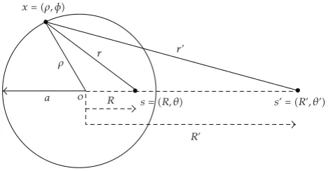
s’ R’, θ’ s R, θ

R’

R o a

ρ r

r’

x ρ, φ

Figure 1:Method of reciprocal radii.

In the potential theory, it is well known that the image method can solve potential problems when the fundamental solution is known. The image point was found in a semi-inverse method a priori through the reciprocal radii in the Sommerfeld’s book4as shown inFigure 1. Sommerfeld and Greenberg 5 both utilized the concept of reciprocal radii of Thomson6to derive the Poisson integral formula. It is important to find where the location of image point is. However, we do not find a natural and logical way about how to determine the location of image point in the literature until an alternative way proposed by Chen and Wu7. Chen and Wu derived the location of image point for a source singularity in a straightforward way through the use of degenerate kernel and proved an alterative way to derive the Poisson integral formula. The fundamental solutions of source singularity are expanded into degenerate kernels for constructing the Green’s function. Since the degenerate kernel separates the source and field points for the closed-form fundamental solution, it plays an important role in studying the image location8,9. To determine the location of image point for screw dislocation in a straightforward way is the main concern of the present paper. In this paper, we will introduce the degenerateor so-called separablekernel for the angle-based fundamental solutionψfor the screw dislocation instead of radial-basis one

lnrfor the source singularity. By employing the degenerate kernel, the closed-form Green’s function is expanded into the degenerate form. Also, the location of image point is found in a straightforward way. The two-dimensional Laplace exterior problems are solved. Finally, two examples were given to demonstrate the validity of the present method.

2. Degenerate (Separable) Kernel for the Angle-Based

Fundamental Solution

(3)

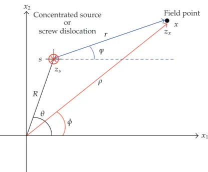
x1 ρ

zs

φ θ R

s

r

x

ψ

zx

Field point

x2

Concentrated source or screw dislocation

Figure 2:Sketch of the concentrated source and the screw dislocation.

Similarly, the field pointxcan be expressed byzx ρeiφin the complex plane as shown in

Figure 2. By decomposing the lnzx−zsinto real and imaginary parts, we have

lnzx−zs ln

reiψlnriψ. 2.1

The real partlnris the fundamental solution of the source singularity while the imaginary partψdenotes the fundamental solution of the screw dislocation. For the exterior caseR < ρ,2.1can be expanded as follows:

lnzx−zs lnzx ln

1− zs

zx

lnρeiφ−

∞

m1 1 m

zs

zx

m

lnρiφ−

∞

m1 1 m

Reiθ ρeiφ

m

lnρiφ−

∞

m1 1 m

R ρ

m

cosmθ−φisinmθ−φ.

2.2

Thus, the degenerate form for the fundamental solution of the screw dislocation,ψs, x, can be expressed as

ψs, x φ−

∞

m1 1 m

R ρ

m

(4)

Similarly, we have

ψs, x θπ

∞

m1 1 m

_ρ R

m

sinmθ−φ, ρ < R, 2.4

for the interior case. InFigure 2, the range ofψs, xis defined between 0 and 2π. To match the physical meaning and mathematical requirement, we modify the range of interest between −πandπ. Thus, the fundamental solution of the screw dislocationψs, xis expressed by

ψs, x ⎧ ⎪ ⎪ ⎪ ⎨ ⎪ ⎪ ⎪ ⎩

ψI_{R, θ}_;_{ρ, φ}_θ∞ m1 1 m

_ρ

R m

sinmθ−φ, ρ < R,

ψE_{R, θ}_;_{ρ, φ}_φ₋_π₋∞ m1 1 m

R ρ

m

sinmθ−φ, ρ > R,

2.5

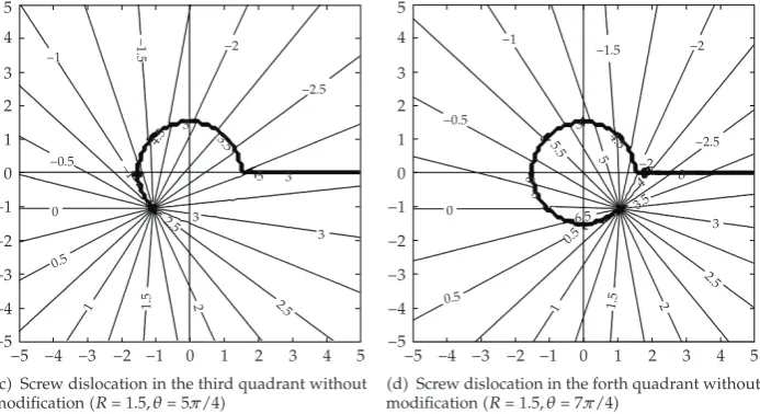
where the superscriptsIandEdenote the interior and exterior cases, respectively. It is noted that the denominator in2.5involves the larger argument to ensure the series convergence. The displacement contour of the screw dislocation in the four quadrants by using 2.5is shown in Figures3a–3d. When the screw dislocation locates at the four quadrants, there are certain areas falling outside the range between −π and π. We subtract 2π, where the value is greater than π to ensure the value in the range. Similarly, we add 2π, where the value is smaller than −π. When the response falls in the defined range, Figure 4 shows the displacement contour for the screw dislocation. To the authors’ best knowledge, the degenerate kernel for the angle-based fundamental solution was not found in the literature.

3.

2 D Exterior Problem

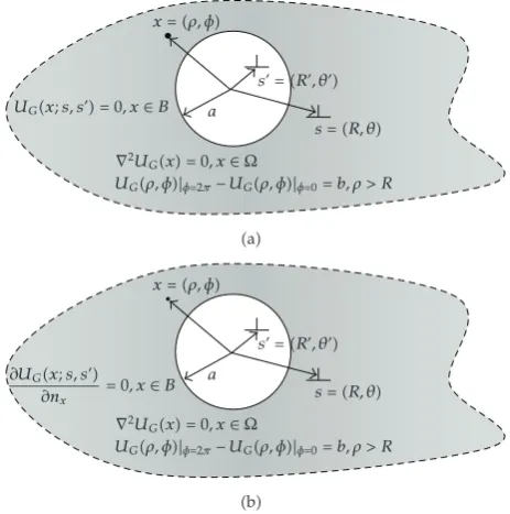
For the problem of an infinite plane problem with a circular boundary under the screw dislocation as shown inFigure 5a, the function of displacement field satisfies

∇2_U

Gx 0, x∈Ω,

UG

ρ, φ|_φ₂_π−UG

ρ, φ|_φ₀b, ρ > R, 3.1

whereΩis the domain of interest andbis the Burger’s vector which is equal to 2π in this paper. The boundary condition on the circular boundary is the Dirichlet type

UGx|x∈BUG

ρ, φ|_ρ_a0, 3.2

whereais the radius of the circular boundary andBis the circular boundary. By employing the image method, the image point is located outside the domain and the solution can be represented as follows:

UG

(5)

−5 −4 −3 −2 −1 0 1 2 3 4 5

−5

−4

−3

−2

−1 0 1 2 3 4 5

−0.5 −1 ₋1.5 −2

−2.5

−3

−3.5

2.5

2 2 2

1.5

1

.

5

1 1

0.5

0 0

−0.5

−4

a Screw dislocation in the first quadrant without modificationR1.5, θπ/4

−5 −4 −3 −2 −1 0 1 2 3 4 5

−5

−4

−3

−2

−1 0 1 2 3 4 5

−1 −1_.

5 −2 −2.5

−3

0

2.5

2

2.5 3

1

.

5

1

.

5

2

1 1 0.5 −0.5

0

0 3.5

5

b Screw dislocation in the second quadrant with-out modificationR1.5, θ3π/4

−5 −4 −3 −2 −1 0 1 2 3 4 5

−5

−4

−3

−2

−1 0 1 2 3 4 5

−1

−

1

.

5 −2

−2.5

3

2_.₅

3

3_. 5

1

.

5 ₂

0.5

−₁

2_.₅

0

3

−0.5

4.5

5

1

c Screw dislocation in the third quadrant without modificationR1.5, θ5π/4

−5 −4 −3 −2 −1 0 1 2 3 4 5

−5

−4

−3

−2

−1 0 1 2 3 4 5

−1

−1.5 −2

−2.5 3

3

2_.5

2 6.5

4_.₅

1 1.5

0.5

0

6

0.5

0

3

−0.5

5_. 5

−2

3.5 4 5

dScrew dislocation in the forth quadrant without modificationR1.5, θ7π/4

Figure 3:Screw dislocation inathe first,bthe second,cthe third, anddthe forth quadrant without

modification.

wheresis the location of image point,cis a free constant, and

ψs, x θ

∞

m1 1 m

_ρ R

m

sinmθ−φ, ρ < R,

ψs, xφ−π−

∞

m1 1 m

R

ρ

m

sinmθ−φ, ρ > R.

(6)

−5 −4 −3 −2 −1 0 1 2 3 4 5

−5

−4

−3

−2

−1 0 1 2 3 4 5

−1

−0.5

−

1

.

5 −2

−2.5

3 3 2.5 3

2.5

−3

2 2 2

1.5 1.5 0,0

1

−0.5

1 0.5

0 0

Figure 4:Screw dislocation in the first quadrant after modificationR1.5,θπ/4.

s R, θ

s’ R’, θ’

a UGx;s, s’ 0, x∈B

x ρ, φ

∇2_U

Gx 0, x∈Ω

UGρ, φ|φ2π−UGρ, φ|φ0b, ρ > R

a

s R, θ s’ R’, θ’

a ∂UGx;s, s’

∂nx

0, x∈B x ρ, φ

∇2_U

Gx 0, x∈Ω

UGρ, φ|φ2π−UGρ, φ|φ0b, ρ > R

b

Figure 5:2D exterior problemaDirichlet boundary condition andbNeumann boundary condition.

In order to match the boundary condition and the Burger’s vector, first the sum of series is independent ofφ. Therefore, we choose the collinear pointssands, that is,θ θand we have

∞

m1 1 m

_a

R m

sinmθ−φ−

∞

m1 1 m

R

a

m

(7)

Finally, we can obtain the location of image point

R

a

a R ⇒R

ρ2

R

a2

R, 3.6

ψs, x ψs, xθφ−π. 3.7

Second, we found thatcis equal to−θ−φπand the solutionUGx;s, sautomatically

matches the boundary condition and Burger’s vector. The displacement field of the closed-form Green’s function can be obtained as below

UG

x;s, sψs, x ψs, x−θ−φπ. 3.8

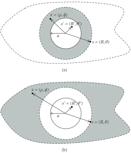
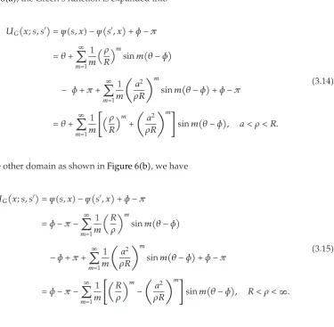
For the domaina < ρ < Ras shown inFigure 6a, the Green’s function is expanded into

UG

x;s, sψs, x ψs, x−θ−φπ

θ

∞

m1 1 m

_ρ

R m

sinmθ−φ

φ−π−

∞

m1 1 m

a2 ρR

m

sinmθ−φ−θ−φπ

∞

m1 1 m

_ρ

R m

−

a2 ρR

m

sinmθ−φ, a < ρ < R.

3.9

Similarly, the Green’s function in the other regionR < ρ <∞is shown inFigure 6band is expanded into

UG

x;s, sψs, x ψs, x−θ−φπ

φ−π−

∞

m1 1 m

R ρ

m

sinmθ−φ

φ−π−

∞

m1 1 m

a2 ρR

m

sinmθ−φ−θ−φπ

φ−θ−π−

∞

m1 1 m

R ρ

m

a2 ρR

m

sinmθ−φ, R < ρ <∞.

(8)

s R, θ s’ R’, θ’

a x ρ, φ

a

s R, θ

s’ R’, θ’ a

x ρ, φ

b

Figure 6:Green’s function ofathe inner domaina < ρ < Randbthe outer domainR < ρ <∞for

the exterior problem.

For comparison, the closed-form solution of Smith’s solution is expressed in terms of functions of complex variables

Fz μEb

2πilogz−z0 μEb

2πilog

a2 z −z0

,

UGx

1 μE

ReFz,

3.11

whereFzandμEdenote the complex function and shear modulus, respectively,z0denotes

the conjugate of the position vector of the screw dislocation, and Re·denotes the real part. Figures7aand7bshow the contour of displacement field by using the Smith’s method

1and the present approach, respectively. Good agreement is made.

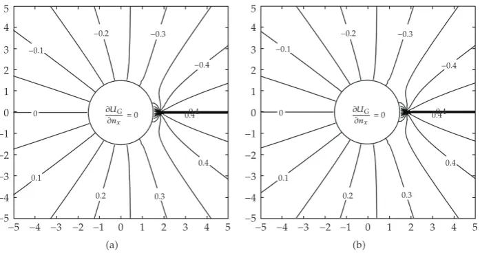
According to the successful experience of the Dirichlet boundary condition for the exterior problem, we extend our approach to the Neumann boundary condition, as shown in

Figure 5b,

∂UGx

∂nx

x∈B

∂UG

ρ, φ ∂ρ

ρa

(9)

Ta b le 1: Comparison for the sour ce or sink and the scr ew d islocation Dirichlet B .C . . Sour ce or sink Chen and W u 7 Scr ew d islocation pr esent p aper ln z ln r iψ ln r ψ

Exterior problem Dirichlet

B .C . s R, θ s ’ R ’ ,θ ’ R ’ a 2 _R a UG x ; s, s ’ 0 ,x ∈ B x ρ, φ ∇ 2U G x δ x − s − δ x − s ’ ,x ∈ Ω s R, θ s ’ R ’ ,θ ’ R ’ a 2 _R a UG x ; s, s ’ 0 ,x ∈ B x ρ, φ ∇ 2U G x 0 ,x ∈ Ω UG ρ, φ |φ 2 π − UG ρ, φ |φ 0 b, ρ > R The closed form UG x ; s, s ln | x − s |− ln | x − s | ln a − ln R UG x ; s, s φ s, x φ s ,x − θ − φ π UG x ; s, s UG x ; s, s The series form ⎧ ⎪ ⎪ ⎪ ⎪ ⎨ ⎪ ⎪ ⎪ ⎪ ⎩ ln a ρ −

∞ _m1

1 m ρ R m − a 2 ρR m cos m θ − φ ,a < ρ < R ln a R −

∞ _m1

1 _m R ρ m − a 2 ρR m cos m θ − φ , R<ρ < ∞ ⎧ ⎪ ⎪ ⎪ ⎪ ⎨ ⎪ ⎪ ⎪ ⎪ ⎩

∞ _m1

1 m ρ R m − a 2 ρR m sin m θ − φ , a <ρ <R φ − θ − π −

∞ _m1

1 m R ρ m a 2 ρR m sin m θ − φ , R<ρ < ∞ Smith’s solution F z μE b 2 π i log z − z0 μE b 2 π i log

⎛ a⎜ ⎝

2 − _z

z0 ⎞ ⎟ ⎠ UG x

1 _μE

Im F z F z μE b 2 πi log z − z0 μE b 2 πi log

⎛ a⎜ ⎝

2 − _z

z0 ⎞ ⎟ ⎠ UG x

1 _μE

(10)

Ta b le 2: Comparison for the sour ce or sink and the scr ew d islocation Neumann B .C. . Sour ce or sink Chen and W u 7 Scr ew d islocation pr esent p aper ln z ln r iψ ln r ψ

Exterior problem Neumann

B . C. s R, θ s ’ R ’ ,θ ’ R ’ a 2 _R a ∂U G x ; s, s ’ ∂n x 0 ,x ∈ B x ρ, φ ∇ 2U G x δ x − s − δ x − s ’ ,x ∈ Ω s R, θ s ’ R ’ ,θ ’ R ’ a 2 _R a ∂U G x ; s, s ’ ∂n x 0 ,x ∈ B x ρ, φ ∇ 2U G x 0 ,x ∈ Ω UG ρ, φ |φ 2 π − UG ρ, φ |φ 0 b, ρ > R The closed form UG x ; s, s ln | x − s | ln | x − s |− ln ρ UG x ; s, s φ s, x − φ s ,x φ − π. UG x ; s, s UG x ; s, s The series form ⎧ ⎪ ⎪ ⎪ ⎪ ⎨ ⎪ ⎪ ⎪ ⎪ ⎩ ln R −

∞ _m1

1 m ρ R m a 2 ρR m cos m θ − φ , a<ρ <R ln ρ −

∞ _m1

1 m R ρ m a 2 ρR m cos m θ − φ , R<ρ < ∞ ⎧ ⎪ ⎪ ⎪ ⎪ ⎨ ⎪ ⎪ ⎪ ⎪ ⎩ θ

∞ _m1

1 _m ρ R m a 2 ρR m sin m θ − φ , a<ρ <R φ − π −

∞ _m1

1 _m R ρ m − a 2 ρR m sin m θ − φ ,R < ρ < ∞ Smith’s solution F z μE b 2 π i log z − z0 − μE b 2 π i log

⎛ a⎜ ⎝

2 − _z

z0 ⎞ ⎟ ⎠ UG x

1 Im _μE

F z F z μE b 2 π i log z − z0 − μE b 2 π i log

⎛ a⎜ ⎝

2 − _z

z0 ⎞ ⎟ ⎠ UG x

1 _μE

(11)

−5 −4 −3 −2 −1 0 1 2 3 4 5

−5

−4

−3

−2

−1 0 1 2 3 4 5

−0.1

−0.2 −0.3

−0.4 0.4 0.4

0.4

0.3

0_. 3

0

.

2

0.1

UG0

0

−₀ .1

a

−5 −4 −3 −2 −1 0 1 2 3 4 5

−5

−4

−3

−2

−1 0 1 2 3 4 5

−0.1

−0.2 −0.3

−0.4 0.4 0.4

0.4

0.3

0_. 3

0

.

2

0.1

UG0

0

−₀ .1

b

Figure 7:Displacement contourDirichlet boundary conditionby usingathe Smith’s method1and

bthe present methodM50.

−5 −4 −3 −2 −1 0 1 2 3 4 5

−5

−4

−3

−2

−1 0 1 2 3 4 5

−0.2

−0.1

−0.3

−0.4

0.4 0.4

0.4

0.3 0.2

0.1

∂UG

∂nx 0

0

a

−5 −4 −3 −2 −1 0 1 2 3 4 5

−5

−4

−3

−2

−1 0 1 2 3 4 5

−0.2

−0.1

−0.3

−0.4

0.4 0.4

0.4

0.3 0.2

0.1

∂UG

∂nx 0

0

b

Figure 8:Displacement contourNeumann boundary conditionby usingathe Smith’s method1and

bthe present methodM50.

In a similar way, we have the closed-form Green’s function for the Neumann boundary condition as

UG

(12)

and the series form is expressed into two parts. For the domain a < ρ < Ras shown in

Figure 6a, the Green’s function is expanded into

UG

x;s, sψs, x−ψs, xφ−π

θ

∞

m1 1 m

_ρ

R m

sinmθ−φ

− φπ

∞

m1 1 m

a2 ρR

m

sinmθ−φφ−π

θ

∞

m1 1 m

_ρ

R m

a2 ρR

m

sinmθ−φ, a < ρ < R.

3.14

For the other domain as shown inFigure 6b, we have

UG

x;s, sψs, x−ψs, xφ−π

φ−π−

∞

m1 1 m

R ρ

m

sinmθ−φ

−φπ

∞

m1 1 m

a2 ρR

m

sinmθ−φφ−π

φ−π−

∞

m1 1 m

R ρ

m

−

a2 ρR

m

sinmθ−φ, R < ρ <∞.

3.15

For comparison, the closed-form solution of Smith’s solution is expressed in terms of functions of complex variable

Fz μEb

2πilogz−z0− μEb

2πilog

a2 z −z0

,

UGx

1 μE

ReFz.

3.16

Figures8aand8bshow the contour of displacement field by using the Smith’s method

(13)

4. Conclusions

For the screw dislocation problem with circular boundaries, we have proposed a natural approach to construct the screw dislocation solution by using the degenerate kernel. The angle-based fundamental solution for screw dislocation was derived in terms of degenerate kernel in this paper. Based on this expression, the image location can be determined instead of using reciprocal radius. Two examples, including an infinite plane with a circular hole subject to the Dirichlet and Neumann boundary conditions, were used to demonstrate the validity of the present formulation.

Acknowledgments

The financial support from the National Science Council under Grant no. NSC-98-2221-E-019-017-MY3 for National Taiwan Ocean University is gratefully appreciated. Thanks to Mr. S. R. Yu for preparing the figures.

References

1 E. Smith, “The interaction between dislocations and inhomogeneities-I,” International Journal of Engineering Science, vol. 6, no. 3, pp. 129–143, 1968.

2 J. Dundurs, “Elastic interaction of dislocations with inhomogeneities,” in Mathematical Theory of Dislocations, T. Mura, Ed., pp. 70–115, American Society of Mechanical Engineers, New York, NY, USA, 1969.

3 G. P. Sendeckyj, “Screw dislocations near circular inclusions,”Physica Status Solidi, vol. 30, pp. 529–535, 1970.

4 A. Sommerfeld,Partial Diﬀerential Equations in Physics, Academic Press, New York, NY, USA, 1949. 5 M. D. Greenbreg,Application of Green’s Functions in Science and Engineering, Prentice-Hill, Upper Saddle

River, NJ, USA, 1971.

6 W. Thomson,Maxwell in His Treatise, vol. 1, chapter 11, Oxford University Press, Oxford, UK, 1848. 7 J. T. Chen and C. S. Wu, “Alternative derivations for the poisson integral formula,”International Journal

of Mathematical Education in Science and Technology, vol. 37, no. 2, pp. 165–185, 2006.

8 J. T. Chen, H. C. Shieh, Y. T. Lee, and J. W. Lee, “Image solutions for boundary value problems without sources,”Applied Mathematics Computation, vol. 216, pp. 1453–1468, 2010.