Complexity of Equivalence and Learning for Multiplicity
Tree Automata
Ines Maruˇsi´c [email protected]
James Worrell [email protected]
Department of Computer Science University of Oxford
Parks Road, Oxford OX1 3QD, UK
Editor:Alexander Clark
Abstract
We consider the query and computational complexity of learning multiplicity tree au-tomata in Angluin’s exact learning model. In this model, there is an oracle, called the Teacher, that can answer membership and equivalence queries posed by the Learner. Mo-tivated by this feature, we first characterise the complexity of the equivalence problem for multiplicity tree automata, showing that it is logspace equivalent to polynomial identity testing.
We then move to query complexity, deriving lower bounds on the number of queries needed to learn multiplicity tree automata over both fixed and arbitrary fields. In the latter case, the bound is linear in the size of the target automaton. The best known upper bound on the query complexity over arbitrary fields derives from an algorithm of Habrard and Oncina (2006), in which the number of queries is proportional to the size of the target automaton and the size of a largest counterexample, represented as a tree, that is returned by the Teacher. However, a smallest counterexample tree may already be exponential in the size of the target automaton. Thus the above algorithm has query complexity exponentially larger than our lower bound, and does not run in time polynomial in the size of the target automaton.
We give a new learning algorithm for multiplicity tree automata in which counterex-amples to equivalence queries are represented as DAGs. The query complexity of this algorithm is quadratic in the target automaton size and linear in the size of a largest coun-terexample. In particular, if the Teacher always returns DAG counterexamples of minimal size then the query complexity is quadratic in the target automaton size—almost matching the lower bound, and improving the best previously-known algorithm by an exponential factor.
Keywords: exact learning, query complexity, multiplicity tree automata, Hankel matri-ces, DAG representations of trees, polynomial identity testing
1. Introduction
general functions from trees into the real numbers. A broad class of such functions can be defined by multiplicity tree automata, a powerful algebraic model which strictly generalises probabilistic tree automata.
Multiplicity tree automata were introduced by Berstel and Reutenauer (1982) under the terminology of linear representations of tree series. They augment classical finite tree automata by assigning to each transition a value in a field. They also generalise multiplicity word automata, introduced by Sch¨utzenberger (1961), since words are a special case of trees. Multiplicity tree automata define many natural structural properties of trees and can be used to model probabilistic processes running on trees. Multiplicity word and tree automata have been applied to a wide variety of machine learning problems, including speech recognition, image processing, character recognition, and grammatical inference; see the paper of Balle and Mohri (2012) for references.
The task of learning automata from examples and queries has been extensively studied since the 1960s. Two notable results in this domain show the impossibility of efficiently learning deterministic finite automata from positive and negative examples alone. First, Gold (1978) showed that the problem of exactly identifying the smallest deterministic finite automaton consistent with a set of accepted and rejected words is NP-hard. Later, Kearns and Valiant (1994) showed that the concept class of regular languages is not efficiently PAC learnable using any polynomially-evaluable hypothesis class under standard cryptographic assumptions.
A significant positive result on learning regular languages was achieved by Angluin (1987), who considered a Learner that did not just passively receive data but that was also able to ask queries. Specifically, Angluin consideredmembership queries, in which the Learner asks an oracle whether a given word belongs to the target language, andequivalence
queries, in which the Learner asks an oracle whether a hypothesis is correct, obtaining a
counterexample if it is not. Subsequent research has sought to establish the learnability of many other hypothesis classes in the same setting, including classes of Boolean formulae, decision trees, context-free languages, and polynomials; see the book of Kearns and Vazirani (1994, Chapter 8) for more details and references.
In this paper we study the problem of learning multiplicity tree automata in the exact
learning modelof Angluin (1988), outlined above. Formally, in this model a Learner actively
collects information about the target function from a Teacher throughmembership queries, which ask for the value of the function on a specific input, and equivalence queries, which suggest a hypothesis to which the Teacher provides a counterexample if one exists. A class of functionsC isexactly learnable if there exists an exact learning algorithm such that for any function f ∈ C, the Learner identifies f using polynomially many membership and equivalence queries in the size of a shortest representation of f and the size of a largest counterexample returned by the Teacher during the execution of the algorithm. The exact learning model is an important theoretical model of the learning process. It is well known that learnability in the exact learning model also implies learnability in the PAC model with membership queries (Valiant, 1985).
equivalence of multiplicity tree automata is decidable in polynomial time assuming unit-cost arithmetic, and in randomised polynomial time in the usual bit-cost model. No finer analysis of the complexity of this problem exists to date. In contrast, the complexity of equivalence for classical nondeterministic word and tree automata has been completely characterised: PSPACE-complete over words (Aho et al., 1974) and EXPTIME-complete over trees (Seidl, 1990).
Our first contribution, in Section 3, is to show that the equivalence problem for multi-plicity tree automata is logspace equivalent to polynomial identity testing, i.e., the problem of deciding whether a polynomial given as an arithmetic circuit is zero. The latter problem is known to be solvable in randomised polynomial time (DeMillo and Lipton, 1978; Schwartz, 1980; Zippel, 1979), whereas solving it in deterministic polynomial time is a well-studied and longstanding open problem (see Arora and Barak, 2009).
Our second contribution, in Section 5, is to give lower bounds on the number of queries needed to learn multiplicity tree automata in the exact learning model, both for the case of an arbitrary and a fixed underlying field. The bound in the former case is linear in the automaton size. In the latter case, the bound is linear in the automaton size for alphabets of a fixed maximal rank. To the best of our knowledge, these are the first lower bounds on the query complexity of exactly learning multiplicity tree automata.
Habrard and Oncina (2006) give an algorithm for learning multiplicity tree automata in the exact learning model. Consider a target multiplicity tree automaton whose minimal representation A has n states. The algorithm of Habrard and Oncina, op. cit., makes at mostnequivalence queries and number of membership queries proportional to|A| ·s, where
|A|is the size of A and s is the size of a largest counterexample returned by the Teacher. Since this algorithm assumes that the Teacher returns counterexamples represented explic-itly as trees, s can be exponential in |A|, even for a Teacher that returns counterexamples of minimal size (see Example 3). This observation reveals an exponential gap between the query complexity of the algorithm of Habrard and Oncina (2006) and our above-mentioned lower bound, which is only linear in |A|. Another consequence is that the worst-case time complexity of this algorithm is exponential in the size of the target automaton.
Given two inequivalent multiplicity tree automata with n states in total, the algorithm of Seidl (1990) produces a subtree-closed set of trees of cardinality at mostnthat contains a tree on which the automata differ. It follows that the counterexample contained in this set has at mostnsubtrees, and hence can be represented as a DAG with at mostnvertices (see Section 3.2). Thus in the context of exact learning it is natural to consider a Teacher that can return succinctly-represented counterexamples, i.e., trees represented as DAGs.
In Section 4, we present a new exact learning algorithm for multiplicity tree automata that achieves the same bound on the number of equivalence queries as the algorithm of Habrard and Oncina (2006), while using number of membership queries quadratic in the target automaton size and linear in the largest counterexample size, even when counterex-amples are given as DAGs. Assuming that the Teacher provides minimal DAG representa-tions of counterexamples, our algorithm therefore makes quadratically many queries in the target automaton size. This is exponentially fewer queries than the best previously-known algorithm (Habrard and Oncina, 2006) and quadratic in the above-mentioned lower bound. Furthermore, our algorithm performs a quadratic number of arithmetic operations in the size of the target automaton, and can be implemented in randomised polynomial time in the Turing model.
Like the algorithm of Habrard and Oncina (2006), our algorithm constructs a matricial representation of the target automaton, called the Hankel matrix (Carlyle and Paz, 1971; Fliess, 1974). However on receiving a counterexample tree z, the former algorithm adds a new column to the Hankel matrix for every suffix of z, while our algorithm adds (at most) one new row for each subtree of z. Crucially the number of suffixes may be exponential in the size of a DAG representation of z, whereas the number of subtrees is only linear in the size of a DAG representation.
An extended abstract (Maruˇsi´c and Worrell, 2014) of this work appeared in the proceed-ings of MFCS 2014. The current paper contains full proofs of all results reported there, the formal definition of multiplicity tree automata running on DAGs, and a refined complexity analysis of the learning algorithm.
1.1 Related Work
One of the earliest results about the exact learning model was the proof of Angluin (1987) that deterministic finite automata are learnable. This result was generalised by Drewes and H¨ogberg (2007) to show exact learnability of deterministic finite (bottom-up) tree automata, generalising also a result of Sakakibara (1990) on the exact learnability of context-free grammars from their structural descriptions1.
The learning algorithm of Drewes and H¨ogberg (2007) was generalised by Maletti (2007) to show that deterministic weighted tree automata over a (commutative) semifield are ex-actly learnable, generalising also an earlier result of Drewes and Vogler (2007) which was restricted to the class of deterministic all-accepting (i.e., every final weight is non zero) weighted tree automata. Recently, a unifying framework for exact learning of deterministic weighted tree automata over a semifield has been proposed (Drewes et al., 2011). Specifi-cally, Drewes et al.,op. cit., introduce the notion of abstract observation tables, an abstract data type for learning deterministic weighted tree automata in the exact learning model, and show that every correct implementation of abstract observation tables yields a correct learning algorithm.
Exact learnability of nondeterministic weighted automata over a field (here called
mul-tiplicity automata) has also been extensively studied. Beimel et al. (2000) show that
mul-tiplicity word automata can be learned efficiently, and apply this to learn various classes of DNF formulae and polynomials. These results were generalised by Klivans and Shpilka
(2006) to show exact learnability of restricted algebraic branching programs and noncom-mutative set-multilinear arithmetic formulae. Bisht et al. (2006) give an almost tight (up to a log factor) lower bound on the number of queries made by any exact learning algorithm for the class of multiplicity word automata.
An exact learning algorithm for a class of nondeterministic tree automata, namely
resid-ual finite tree automata, is given by Kasprzik (2013). The latter paper identifies the size
of counterexamples as a hidden exponential factor in the complexity of the learning algo-rithm, observing in particular that a smallest counterexample can have exponential size in the number of states of the target automaton. Such a phenomenon does not prevent the class of tree automata from being exactly learnable since in the exact learning model the complexity measure takes into account the size of a largest counterexample. However, this does raise the question of developing a learning algorithm whose complexity would be polynomial in the size of succinctly-represented counterexamples, which is one of the motivations for the present work.
Denis and Habrard (2007) consider the problem of learning probability distributions over trees that are recognised by a multiplicity tree automaton from samples drawn in-dependently according to the target distribution. They give an inference algorithm that exactly identifies such recognisable probability distributions in the limit with probability one (with respect to the randomly-drawn examples). Most closely related to the topic of the present paper is the work of Habrard and Oncina (2006), who give an algorithm for learning multiplicity tree automata in the exact learning model, as discussed above.
A variety of spectral methods have been employed for learning multiplicity word and tree automata (Bailly et al., 2009; Balle and Mohri, 2012; Denis et al., 2014; Gybels et al., 2014). This line of research originates in earlier work of Hsu et al. (2012) that gives a spectral learning algorithm (based on singular value decomposition) for hidden Markov models. Particularly close to the present paper is the work of Bailly et al. (2010), which learns probability distributions over trees that are recognised by some multiplicity tree automaton. Their approach lies within a passive learning framework in which one is given a sample of trees independently drawn according to a target distribution, and the aim is to infer a multiplicity tree automaton that approximates the target. As in our approach, the notion of a Hankel matrix plays a central role in the algorithm of Bailly et al. (2010). There the Hankel matrix is called an observation matrix, and it encodes an empirical distribution on trees obtained by sampling from the target distribution. Bailly et al., op. cit., apply principal component analysis in order to identify a low-dimensional approximation of the vector space spanned by the residuals of the target probability distribution. From this approximation they build an automaton whose associated tree series approximates the target distribution. They moreover obtain bounds on the estimation error of the output tree series with respect to the target distribution in terms of the sample size and the desired confidence.
In contrast to the above-described approach of Bailly et al. (2010), in our work the target dimension (i.e., number of states) is not part of the input since our aim is to learn aminimal
2. Preliminaries
Let N and N0 denote the set of all positive and nonnegative integers, respectively. Let
n ∈ N. We write [n] for the set {1,2, . . . , n} and In for the identity matrix of order n. For every i ∈ [n], we write ei for the ith n-dimensional coordinate row vector. For any
n-dimensional vector v, we writevi for its ith entry.
For any matrixA, we writeAifor itsithrow,Aj for itsjthcolumn, andAi,j for its (i, j)th entry. Given nonempty subsetsIandJ of the rows and columns ofA, respectively, we write
AI,J for the submatrix (Ai,j)i∈I,j∈J ofA. For singletons, we write simplyAi,J :=A{i},J and
AI,j :=AI,{j}. We also consider matrices whose rows and columns are indexed by tuples of natural numbers ordered lexicographically.
Given a set V, we denote by V∗ the set of all finite ordered tuples of elements from
V. For any subset S ⊆V, thecharacteristic function of S (relative to V) is the function
χS :V → {0,1} such thatχS(x) = 1 ifx∈S, and χS(x) = 0 otherwise.
2.1 Kronecker Product
Let A be a matrix of dimension m1 ×n1 and B a matrix of dimension m2 ×n2. The
Kronecker product of A by B, written as A⊗B, is a matrix of dimension m1m2×n1n2
where (A⊗B)(i1,i2),(j1,j2)=Ai1,j1·Bi2,j2 for everyi1∈[m1],i2∈[m2],j1 ∈[n1],j2 ∈[n2].
The Kronecker product is bilinear, associative, and has the following mixed-product
property: For any matricesA,B, C, Dsuch that products A·C and B·Dare defined, it
holds that (A⊗B)·(C⊗D) = (A·C)⊗(B·D).
Letk∈NandA1, . . . , Akbe matrices such that for everyl∈[k], matrixAlhasnlrows. It can easily be shown using induction on kthat for every (i1, . . . , ik)∈[n1]× · · · ×[nk], it holds that
(A1⊗ · · · ⊗Ak)(i1,...,ik)= (A1)i1 ⊗ · · · ⊗(Ak)ik. (1) We writeNk
l=1Al:=A1⊗ · · · ⊗Ak.
For every k∈N0 we define thek-fold Kronecker power of a matrix A, written as A⊗k, inductively by A⊗0 =I1 andA⊗k=A⊗(k−1)⊗A fork≥1.
Let k∈N0. For any square matricesA andB, we have
(A⊗B)k=Ak⊗Bk. (2)
For any matricesA1, . . . , AkandB1, . . . , Bkwhere productAl·Blis defined for everyl∈[k], we have
(A1⊗ · · · ⊗Ak)·(B1⊗ · · · ⊗Bk) = (A1·B1)⊗ · · · ⊗(Ak·Bk). (3) Equations (2) and (3) follow easily from the mixed-product property by induction onk.
2.2 Finite Trees
A ranked alphabet is a tuple (Σ,rk) where Σ is a nonempty finite set of symbols and
k∈N0, we define the set of all k-ary symbols Σk :=rk−1({k}). If σ∈Σk then we say that
σ has rank (orarity) k. We say that Σ hasrank m ifm=max{rk(σ) :σ∈Σ}.
The set of Σ-trees (trees for short), written as TΣ, is the smallest set T satisfying the following two conditions: (i) Σ0 ⊆ T; and (ii) if k ≥ 1, σ ∈ Σk, t1, . . . , tk ∈ T then
σ(t1, . . . , tk) ∈T. Given a Σ-tree t, asubtree of tis a Σ-tree consisting of a node in t and all of its descendants in t. The set of all subtrees of tis denoted bySub(t).
Let Σ be a ranked alphabet andF be a field. Atree series over Σ with coefficients inF is a functionf :TΣ→F. For everyt∈TΣ, we call f(t) the coefficient of tinf. The set of all tree series over Σ with coefficients in Fis denoted byFhhTΣii.
We define the tree seriesheight,size,#σ ∈QhhTΣiiwhereσ ∈Σ, as follows: (i) ift∈Σ0 then height(t) = 0, size(t) = 1, #σ(t) = χ{t=σ}; and (ii) if t= a(t1, . . . , tk) where k ≥1,
a∈Σk,t1, . . . , tk∈TΣ thenheight(t) = 1 +maxi∈[k]height(ti),size(t) = 1 +Pi∈[k]size(ti), #σ(t) =χ{a=σ}+Pi∈[k]#σ(ti), respectively. For everyn∈N0, we define the sets TΣ<n :=
{t∈TΣ:height(t)< n},TΣn:={t∈TΣ:height(t) =n}, andTΣ≤n:=TΣ<n∪TΣn.
Let 2 be a nullary symbol not contained in Σ. The set CΣ of Σ-contexts (contexts for short) is the set of all ({2} ∪Σ)-trees in which 2 occurs exactly once. Theconcatenation
of c ∈ CΣ and t ∈ TΣ∪˙ CΣ, written as c[t], is the tree obtained by substituting t for 2 in c. Intuitively, the 2-labelled leaf of c acts as a variable in that substituting a Σ-tree (respectively, Σ-context) tfor that variable yields a new Σ-tree (Σ-context)c[t].
A suffix of a Σ-treetis a Σ-contextcsuch thatt=c[t0] for some Σ-treet0. TheHankel matrix of a tree series f ∈FhhTΣiiis the matrix H:TΣ×CΣ→Fsuch that Ht,c=f(c[t]) for everyt∈TΣ and c∈CΣ.
2.3 Multiplicity Tree Automata
LetFbe a field. AnF-multiplicity tree automaton (F-MTA) is a quadrupleA= (n,Σ, µ, γ) which consists of thedimensionn∈N0representing the number of states, a ranked alphabet Σ, a family oftransition matrices µ={µ(σ) :σ∈Σ}, whereµ(σ)∈Fn
rk(σ)×n
, and thefinal weight vector γ ∈Fn×1. The size of the automaton A, written as |A|, is defined as
|A|:= X σ∈Σ
nrk(σ)+1+n.
That is, the size of A is the total number of entries in all transition matrices and the final weight vector.2
Example 1 Let Σ ={0,1,+,×,−}be a ranked alphabet where0,1are nullary symbols and
+,×,− are binary symbols. We define anF-multiplicity tree automaton A= (2,Σ, µ, γ) as
follows. Automaton A has two states, q1 and q2, and has final weight vector γ =
0 1>. This means that states q1 and q2 have final weights γ1 = 0 andγ2 = 1, respectively. Given
a symbol σ ∈Σ of rank k, the transition matrix µ(σ) has dimension 2k×2 and stores the weights of transitions from each k-tuple of origin states to each destination state. Let the
transition matrices of A be µ(0) =
1 0
, µ(1) =
1 1
,
µ(+) =
1 0 0 1 0 1 0 0
, µ(−) =
1 0 0 −1 0 1 0 0
, andµ(×) =
1 0 0 0 0 0 0 1
.
Entryµ(1)2= 1means that there is a transition1→1 q2 with weight1into stateq2on reading
symbol 1. Similarly, entry µ(+)(2,1),2 = 1 means that there is a transition +(q2, q1) 1
→ q2
with weight 1 from pair of states (q2, q1) into state q2 on reading symbol+. We extend µfrom Σ toTΣ by defining
µ(σ(t1, . . . , tk)) := (µ(t1)⊗ · · · ⊗µ(tk))·µ(σ)
for every σ ∈ Σk and t1, . . . , tk ∈ TΣ. The tree series kAk ∈ FhhTΣii recognised by A is defined by kAk(t) =µ(t)·γ for every t ∈ TΣ. Note that a 0-dimensional multiplicity tree automaton necessarily recognises a zero tree series. Two automata A1, A2 are said to be
equivalent ifkA1k ≡ kA2k.
We further extend µ from TΣ to CΣ by treating 2 as a unary symbol and defining
µ(2) :=In. This allows to define µ(c)∈Fn×n for every c=σ(t1, . . . , tk)∈CΣ inductively by writingµ(c) := (µ(t1)⊗ · · · ⊗µ(tk))·µ(σ). It can easily be shown thatµ(c[t]) =µ(t)·µ(c) for everyt∈TΣ and c∈CΣ.
Example 2 Let us consider the computation of F-MTA A = (2,Σ, µ, γ) from Example 1
on the following Σ-treet:
+
×
1 1
+
0 1
The transition matrices define bottom-up runs ofAont. Intuitively, a run ontcorresponds
to multiple copies of automaton A walking along t from leaves to the root. Every such run
has a weight in F which is defined as the product of the weights of all transitions taken.
On tree t, automaton A has one nonzero-weight run ending in state q1, as follows:
+
q1
×
q1
1
q1 q1 1
+
q1
0
Moreover, automaton A has two nonzero-weight runs ending in state q2, as follows: + q2 × q2 1
q2 q2 1
+
q1
0
q1 q1 1
+
q2
×
q1
1
q1 q1 1
+
q2
0
q1 q2 1
Each of the above three runs has weight 1. Therefore, the total weight of all runs of
au-tomatonA on tree t in which the root is labelled q1 is 1, and the total weight of all runs in
which the root is labelled q2 is 2. Indeed, algebraically, by definition ofµ we have that
µ(t) = (µ(×(1,1))⊗µ(+(0,1)))·µ(+)
= (((µ(1)⊗µ(1))·µ(×))⊗((µ(0)⊗µ(1))·µ(+)))·µ(+)
= 1 1 ⊗ 1 1 · 1 0 0 0 0 0 0 1 ⊗ 1 0 ⊗ 1 1 · 1 0 0 1 0 1 0 0 · 1 0 0 1 0 1 0 0 =
1 1 1 1·
1 0 0 0 0 0 0 1 ⊗
1 1 0 0·
1 0 0 1 0 1 0 0 · 1 0 0 1 0 1 0 0
= 1 1⊗
1 1·
1 0 0 1 0 1 0 0
=1 1 1 1·
1 0 0 1 0 1 0 0
=1 2.
Finally, the weight kAk(t) of tree t is the sum of the weights of all runs on t, where the weight of each run is multiplied by the final weight of its root label. Algebraically, we have
kAk(t) =µ(t)·γ =1 2·
0 1> = 2.
Let A1 = (n1,Σ, µ1, γ1) and A2 = (n2,Σ, µ2, γ2) be two F-multiplicity tree automata. Theproduct ofA1byA2, written asA1×A2, is theF-multiplicity tree automaton (n,Σ, µ, γ) where:
• n=n1·n2;
• Ifσ∈Σkthenµ(σ) =Pk·(µ1(σ)⊗µ2(σ)) wherePk is a permutation matrix of order (n1·n2)k uniquely defined (see Remark 1 below) by
• γ =γ1⊗γ2.
Remark 1 We argue that for every k ∈ N0 such that k is the rank of a symbol in Σ, matrixPk is well-defined by Equation (4). In order to do this, it suffices to show that Pk is
well-defined on a set of basis vectors of F1×n1 and F1×n2 and then extend linearly. To that
end, let(e1i)i∈[n1]and (e
2
j)j∈[n2]be bases of F
1×n1 and
F1×n2, respectively. Let us define sets
of vectors
E1 :={(e1i1 ⊗ · · · ⊗e
1 ik)⊗(e
2
j1 ⊗ · · · ⊗e
2
jk) :i1, . . . , ik∈[n1], j1, . . . , jk∈[n2]}
and
E2 :={(e1i1 ⊗e
2
j1)⊗ · · · ⊗(e
1 ik⊗e
2
jk) :i1, . . . , ik ∈[n1], j1, . . . , jk ∈[n2]}.
Then, E1 and E2 are two bases of the vector space F1×n1n2. Therefore, P
k is well-defined
as an invertible matrix mapping basis E1 to basis E2.
Essentially the same product construction as in the proof of the first part of the following proposition is given by Berstel and Reutenauer (1982, Proposition 5.1) using the terminology of linear representations of tree series rather than multiplicity tree automata.
Proposition 2 Let A1 and A2 be F-multiplicity tree automata over a ranked alphabet Σ.
Then, for every t∈TΣ it holds thatkA1×A2k(t) =kA1k(t)· kA2k(t). Furthermore, in case
F=Q, automatonA1×A2 can be computed fromA1 andA2 in logarithmic space.
Proof Let A1 = (n1,Σ, µ1, γ1), A2 = (n2,Σ, µ2, γ2), and A1×A2 = (n,Σ, µ, γ). First we show that for any t∈TΣ,
µ(t) =µ1(t)⊗µ2(t). (5)
We prove that Equation (5) holds for all t ∈ TΣ using induction on height(t). The base case t=σ∈Σ0 holds immediately by definition since P0 =I1. For the induction step, let
h ∈N0 and assume that Equation (5) holds for every t∈TΣ≤h. Take any t∈TΣh+1. Then
t =σ(t1, . . . , tk) for some k ≥ 1, σ ∈Σk, and t1, . . . , tk ∈ TΣ≤h. By induction hypothesis, Equation (4), and the mixed-product property of Kronecker product we now have
µ(t) = (µ(t1)⊗ · · · ⊗µ(tk))·µ(σ)
= ((µ1(t1)⊗µ2(t1))⊗ · · · ⊗(µ1(tk)⊗µ2(tk)))·Pk·(µ1(σ)⊗µ2(σ)) = ((µ1(t1)⊗ · · · ⊗µ1(tk))⊗(µ2(t1)⊗ · · · ⊗µ2(tk)))·(µ1(σ)⊗µ2(σ)) = ((µ1(t1)⊗ · · · ⊗µ1(tk))·µ1(σ))⊗((µ2(t1)⊗ · · · ⊗µ2(tk))·µ2(σ)) =µ1(t)⊗µ2(t).
This completes the proof of Equation (5) by induction. For everyt∈TΣ, we now have
kA1×A2k(t) =µ(t)·γ = (µ1(t)⊗µ2(t))·(γ1⊗γ2)
Automaton A1×A2 can be computed by a Turing machine which scans the transition matrices and the final weight vectors ofA1 andA2, and then writes down the entries of the transition matrices and the final weight vector of their product A1×A2 onto the output tape. This computation requires maintaining only a constant number of counters to store the indices of transition matrices, which takes logarithmic space in the representation of automataA1andA2. Hence, the Turing machine computingA1×A2 uses logarithmic space in the work tape.
A tree seriesf is calledrecognisable if it is recognised by some multiplicity tree automa-ton; such an automaton is called anMTA-representation of f. An MTA-representation of
f that has the smallest dimension is called minimal. The set of all recognisable tree series inFhhTΣiiis denoted by Rec(Σ,F).
The following result was first shown by Bozapalidis and Louscou-Bozapalidou (1983); an essentially equivalent result was later shown by Habrard and Oncina (2006).
Theorem 3 (Bozapalidis and Louscou-Bozapalidou, 1983) Let Σbe a ranked alpha-bet and F be a field. Let f ∈ FhhTΣii and let H be the Hankel matrix of f. It holds that
f ∈Rec(Σ,F)if and only if H has finite rank overF. In casef ∈Rec(Σ,F), the dimension
of a minimal MTA-representation of f equals the rank of H.
The following result by Bozapalidis and Alexandrakis (1989, Proposition 4) states that for any recognisable tree series, its minimal MTA-representation is unique up to change of basis.
Theorem 4 (Bozapalidis and Alexandrakis, 1989) Let Σ be a ranked alphabet and F
be a field. Let f ∈Rec(Σ,F) and let r be the rank (over F) of the Hankel matrix of f. Let
A1 = (r,Σ, µ1, γ1) be an MTA-representation off. Given an F-multiplicity tree automaton
A2 = (r,Σ, µ2, γ2), it holds that A2 recognises f if and only if there exists an invertible
matrix U ∈Fr×r such that γ
2 =U ·γ1 and µ2(σ) =U⊗rk(σ)·µ1(σ)·U−1 for every σ∈Σ. 2.4 DAG Representations of Finite Trees
Adirected multigraphconsists of a set of nodesV and a multiset of directed edgesE⊆V×V. We say that a directed multigraph isacyclic if the underlying directed graph has no cycles; we say it isordered if a linear order on the successors of each node is assumed. A directed multigraph is rooted if there is a distinguished root node v such that all other nodes are reachable fromv.
Let Σ be a ranked alphabet. A DAG representation of a Σ-tree (Σ-DAG orDAG for short) is a rooted acyclic ordered directed multigraph whose nodes are labelled with symbols from Σ such that the outdegree of each node is equal to the rank of the symbol it is labelled with. Formally a Σ-DAG consists of a set of nodesV, for each nodev∈V a list of successors
succ(v) ∈ V∗, and a node labelling λ : V → Σ where for each node v ∈ V it holds that
λ(v)∈Σ|succ(v)|. Note that Σ-trees are a subclass of Σ-DAGs.
of the node v and all of its descendants in G. Clearly, if v is the root of G then G|v =G. The set{G|v :v is a node inG} of all the sub-DAGs of Gis denoted bySub(G).
For any Σ-DAG G, we define its unfolding into a Σ-tree, denoted byunfold(G), induc-tively as follows: If the root of Gis labelled with a symbol σ and has the list of successors
v1, . . . , vk, then
unfold(G) =σ(unfold(G|v
1), . . . ,unfold(G|vk)). The next proposition follows easily from the definition.
Proposition 5 If Gis a Σ-DAG, then Sub(unfold(G)) =unfold[Sub(G)].
Because a context has exactly one occurrence of symbol 2, any DAG representation
of a Σ-context is a ({2} ∪Σ)-DAG that has a unique path from the root to the (unique)
2-labelled node. The concatenation of a DAGK, representing a Σ-context, and a Σ-DAG
Gis the Σ-DAG, denoted byK[G], obtained by substituting the root ofG for2 inK.
Proposition 6 Let K be a DAG representation of a Σ-context, and let G be a Σ-DAG. Then, unfold(K[G]) =unfold(K)[unfold(G)].
Proof The proof is by induction onheight(K). For the base case, letheight(K) = 0. Then, we have that K = 2 and therefore unfold(2[G]) = unfold(G) =unfold(2)[unfold(G)] for any Σ-DAGG.
For the induction step, let h ∈N0 and assume that the result holds ifheight(K) ≤h. Let K be a DAG representation of a Σ-context such that height(K) = h + 1. Let the root of K have label σ and list of successors v1, . . . , vk. By definition, there is a unique path in K going from the root to the 2-labelled node. Without loss of generality, we can assume that the 2-labelled node is a successor of v1. Take an arbitrary Σ-DAG G. Since
height(K|v
1)≤h, we have by the induction hypothesis that
unfold(K[G]) =σ(unfold(K|v
1[G]),unfold(K|v2), . . . ,unfold(K|vk)) =σ(unfold(K|v
1)[unfold(G)],unfold(K|v2), . . . ,unfold(K|vk)) =σ(unfold(K|v
1),unfold(K|v2), . . . ,unfold(K|vk))[unfold(G)] =unfold(K)[unfold(G)].
This completes the proof by induction.
2.5 Multiplicity Tree Automata on DAGs
In this section, we introduce the notion of a multiplicity tree automaton running on DAGs. To the best of our knowledge, this notion has not been studied before.
Let Fbe a field, andA= (n,Σ, µ, γ) be an F-multiplicity tree automaton. The compu-tation of automatonA on a Σ-DAGG= (V, E) is defined as follows: Arun ofA onG is a mapping ρ:Sub(G) →Fn such that for every node v ∈V, if v is labelled withσ and has the list of successors succ(v) =v1, . . . , vk then
ρ(G|v) = (ρ(G|v
Automaton A assigns toG aweight kAk(G)∈F wherekAk(G) =ρ(G)·γ.
In the following proposition, we show that the weight assigned by a multiplicity tree automaton to a DAG is equal to the weight assigned to its tree unfolding.
Proposition 7 Let F be a field, and A= (n,Σ, µ, γ) be an F-multiplicity tree automaton.
For any Σ-DAG G, it holds thatρ(G) =µ(unfold(G)) andkAk(G) =kAk(unfold(G)).
Proof Let V be the set of nodes of G. First we show that for everyv∈V,
ρ(G|v) =µ(unfold(G|v)). (6)
The proof is by induction on height(G|v). For the base case, let height(G|v) = 0. This implies thatG|v =σ∈Σ0. Therefore, by definition we have that
ρ(G|v) =µ(σ) =µ(unfold(σ)) =µ(unfold(G|v)).
For the induction step, let h ∈ N0 and assume that Equation (6) holds for every v ∈ V
such that height(G|v)≤h. Take any v ∈V such that height(G|v) =h+ 1. Let the root of
G|v be labelled with a symbol σ and have list of successors succ(v) =v1, . . . , vk. Then for every j ∈[k], we have that height(G|v
j) ≤h and thus ρ(G|vj) =µ(unfold(G|vj)) holds by the induction hypothesis. This implies that
ρ(G|v) = (ρ(G|v
1)⊗ · · · ⊗ρ(G|vk))·µ(σ) = (µ(unfold(G|v
1))⊗ · · · ⊗µ(unfold(G|vk)))·µ(σ) =µ(σ(unfold(G|v
1), . . . ,unfold(G|vk))) =µ(unfold(G|v)),
which completes the proof of Equation (6) for all v∈V by induction.
Taking v to be the root of G, we get from Equation (6) that ρ(G) = µ(unfold(G)). Therefore, kAk(G) =ρ(G)·γ =µ(unfold(G))·γ =kAk(unfold(G)).
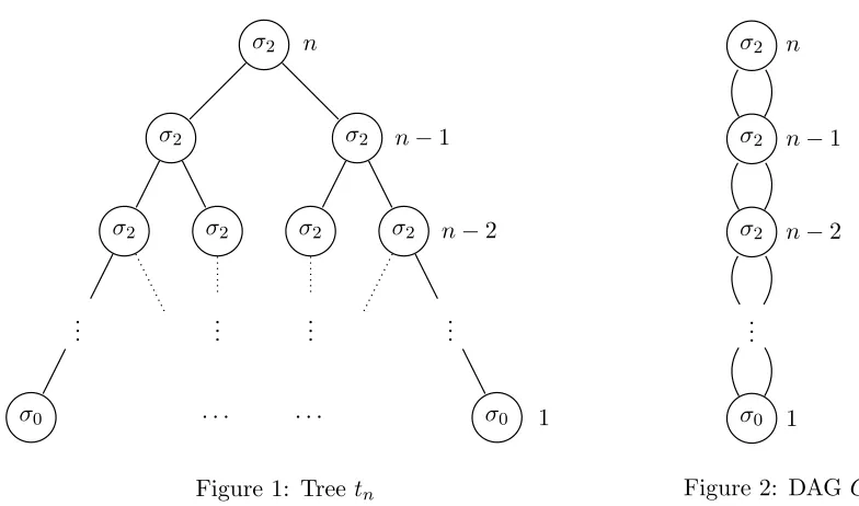
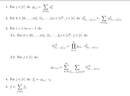
Example 3 Let Σ = {σ0, σ2} be a ranked alphabet such that rk(σ0) = 0 and rk(σ2) = 2.
Take any n∈N. Let tn, depicted in Figure 1, be the perfect binary Σ-tree of height n−1.
Note that size(tn) =O(2n). Define anF-MTAA= (n,Σ, µ, e1)such thatµ(σ0) =en∈F1×n
and µ(σ2)∈Fn2×n
where µ(σ2)(i+1,i+1),i= 1 for every i∈[n−1], and all other entries of
µ(σ2) are zero. It is easy to see thatkAk(tn) = 1 and kAk(t) = 0 for everyt∈TΣ\ {tn}.
Let B be the 0-dimensional F-MTA over Σ (so that kBk ≡ 0). Suppose we were to
check whether automata A and B are equivalent. Then the only counterexample to their
equivalence, namely the treetn, has sizeO(2n). Note, however, thattn has an exponentially
more succinct DAG representation Gn, given in Figure 2.
2.6 Arithmetic Circuits
σ2 n
σ2
σ2
.. .
σ0
σ2
.. .
· · ·
σ2 n−1
σ2
.. .
· · ·
σ2 n−2
.. .
σ0 1
Figure 1: Tree tn
σ0 1 .. .
σ2 n−2
σ2 n−1
σ2 n
Figure 2: DAG Gn
2 are called internal gates and are labelled with an arithmetic operation +, ×, or −. We assume that there is a unique gate with outdegree 0 called the output gate. An arithmetic circuit is called variable-free if all input gates are labelled with 0 or 1.
Given two gates u and v of an arithmetic circuit C, we callu a child of v if (u, v) is a directed edge inC. Thesize ofC is the number of gates inC. Theheight of a gatev inC, written as height(v), is the length of a longest directed path from an input gate to v. The
height of C is the maximal height of a gate in C.
An arithmetic circuit C computes a polynomial over the integers as follows: An input gate of C labelled with α ∈ {0,1} ∪ {xi :i∈N} computes the polynomial α. An internal gate of C labelled with ∗ ∈ {+,×,−} computes the polynomial p1∗p2 where p1 and p2 are the polynomials computed by its children. For any gate v in C, we write fv for the polynomial computed byv. Theoutput ofC, written asfC, is the polynomial computed by the output gate ofC. Thearithmetic circuit identity testing (ACIT)problem asks whether the output of a given arithmetic circuit is equal to the zero polynomial.
Remark 8 Any variable-free arithmetic circuitC can be seen as a Σ-DAG with the ranked alphabet Σ ={0,1,+,×,−}where 0,1 are nullary symbols and+,×,− are binary symbols. Let A= (2,Σ, µ, γ) be the multiplicity tree automaton from Example 1. Then, for any gate
v in C it holds that µ(C|v) =
1 fv
, where C|v is the sub-DAG of C rooted at v and
fv is the number computed at gate v. (This result can be easily proved using induction on
height(C|v).) In particular, when v is the output gate of C we get that
kAk(C) =µ(C)·γ =1 fC
·
0 1> =fC.
2.7 The Learning Model
In this paper we work with the exact learning model of Angluin (1988): Letf be a target
function. ALearner (learning algorithm) may, in each step, propose a hypothesis function
h by making an equivalence query to a Teacher. If h is equivalent to f, then the Teacher returns YES and the Learner succeeds and halts. Otherwise, the Teacher returns NO with a counterexample, which is an assignmentx such that h(x)6=f(x). Moreover, the Learner may query the Teacher for the value of the function f on a particular assignment x by making amembership query onx. The Teacher returns the valuef(x) to such a query.
We say that a class of functions C is exactly learnable if there is a Learner that for any target function f ∈ C, outputs a hypothesis h ∈ C such that h(x) = f(x) for all assignments x, and does so in time polynomial in the size of a shortest representation off
and the size of a largest counterexample returned by the Teacher. We moreover say that the class C is exactly learnable in (randomised) polynomial time if the learning algorithm can be implemented to run in (randomised) polynomial time in the Turing model.
3. Equivalence Queries
In the exact learning model, one of the principal algorithmic questions from the point of view of the Teacher is the computational complexity of equivalence testing. In this section we characterise the computational complexity of equivalence testing for multiplicity tree automata, showing that this problem is logspace equivalent to polynomial identity testing. The latter is a well-studied problem for which there are numerous randomised polynomial-time algorithms, with the existence of a deterministic polynomial-polynomial-time algorithm being a longstanding open problem. Moreover in this section, we explain why it is natural to expect the Teacher to return succinct DAG counterexamples in the case of inequivalence.
3.1 Computational Complexity of MTA Equivalence
A key algorithmic component of the exact learning framework is checking the equivalence of the hypothesis and the target function: a task for the Teacher rather than the Learner. The existence of efficient algorithms to perform such equivalence checks is important for several applications of the exact learning framework (see, e.g., Feng et al., 2011). With this in mind, in this subsection we characterise the computational complexity of the equivalence problem forQ-multiplicity tree automata. Here we specialise the weight field to beQsince we want to work within the classical Turing model of computation. Parts of this section also exploit the fact that Qis an ordered field.
Our main result is:
Theorem 9 The equivalence problem for Q-multiplicity tree automata is logspace
interre-ducible with ACIT.
3.1.1 From MTA Equivalence to ACIT
First, we present a logspace reduction from the equivalence problem forQ-MTAs toACIT. We start with the following lemma.
Lemma 10 Given an integer n∈N and a Q-multiplicity tree automaton A over a ranked
alphabet Σ, one can compute, in logarithmic space in |A| and n, a variable-free arithmetic
circuit that has output P
t∈TΣ<nkAk(t).
Proof Let A= (r,Σ, µ, γ), and let m be the rank of Σ. By definition, it holds that
X
t∈TΣ<n
kAk(t) =
X
t∈TΣ<n
µ(t)
·γ. (7)
We have P
t∈TΣ<1µ(t) =
P
σ∈Σ0µ(σ). Furthermore for everyi∈N, it holds that
TΣ<i+1={σ(t1, . . . , tk) :k∈ {0, . . . , m}, σ∈Σk, t1, . . . , tk∈TΣ<i} and thus by bilinearity of Kronecker product,
X
t∈TΣ<i+1
µ(t) = m X k=0 X σ∈Σk X
t1∈TΣ<i
· · · X
tk∈TΣ<i
(µ(t1)⊗ · · · ⊗µ(tk))·µ(σ)
= m X k=0 X σ∈Σk X
t1∈TΣ<i
µ(t1)
⊗ · · · ⊗
X
tk∈TΣ<i
µ(tk)
·µ(σ)
= m X k=0 X
t∈TΣ<i
µ(t)
⊗k
X
σ∈Σk
µ(σ). (8)
In the following we define a variable-free arithmetic circuit Φ that has outputP
t∈TΣ<nkAk(t). First, let us denote G(i) := P
t∈TΣ<iµ(t) for every i∈ N. Then by Equation (8) we have
G(i+ 1) = Pm
k=0G(i)⊗k ·S(k) where S(k) :=
P
σ∈Σkµ(σ) for every k ∈ {0, . . . , m}. In coordinate notation, for every j∈[r] we have by Equation (1) that
G(i+ 1)j = m
X
k=0
X
(l1,...,lk)∈[r]k
k
Y
a=1
G(i)la·S(k)(l1,...,lk),j. (9)
We present Φ as a straight-line program, with built-in constants
{µσ(l1,...,lk),j, γj :k∈ {0, . . . , m}, σ∈Σk,(l1, . . . , lk)∈[r]k, j ∈[r]}
representing the entries of the transition matrices and the final weight vector ofA, internal variables {sk(l
1,...,lk),j :k ∈ {0, . . . , m},(l1, . . . , lk) ∈ [r]
k, j ∈[r]} and {g
1. Forj∈[r] do g1,j ←
X
σ∈Σ0
µσj
2. Fork∈ {0, . . . , m}, (l1, . . . , lk)∈[r]k,j∈[r] do sk(l1,...,lk),j←
X
σ∈Σk
µσ(l
1,...,lk),j
3. Fori= 1 to n−1 do
3.1. Fork∈ {0, . . . , m}, (l1, . . . , lk)∈[r]k,j∈[r] do
hi,k(l
1,...,lk),j ←
k
Y
a=1
gi,la·s k (l1,...,lk),j
3.2. Forj∈[r] do
gi+1,j← m
X
k=0
X
(l1,...,lk)∈[r]k
hi,k(l
1,...,lk),j
4. Forj∈[r] do fj ←gn,j ·γj
5. f ← X
j∈[r]
fj.
Table 1: Straight-line program Φ
Formally, the straight-line program Φ is given in Table 1. Here the statements are given in indexed-sum and indexed-product notation, which can easily be expanded in terms of the corresponding binary operations. It follows from Equations (7) and (9) that the output of Φ isG(n)·γ =P
t∈TΣ<nkAk(t).
The input gates of Φ are labelled with rational numbers. By separately encoding nu-merators and denominators, we can in logarithmic space reduce Φ to an arithmetic circuit where all input gates are labelled with integers. Moreover, without loss of generality we can assume that every input gate of Φ is labelled with 0 or 1. Any other integer label given in binary can be encoded as an arithmetic circuit.
Recalling that a composition of two logspace reductions is again a logspace reduction, we conclude that the entire computation takes logarithmic space in |A|and n.
Proposition 11 (Seidl, 1990) SupposeAandB are multiplicity tree automata of
dimen-sion n1 and n2, respectively, and over a ranked alphabet Σ. Then, A andB are equivalent
if and only if kAk(t) =kBk(t) for every t∈T<n1+n2
Σ .
We now turn to the reduction:
Proposition 12 The equivalence problem for Q-multiplicity tree automata is logspace
re-ducible toACIT.
Proof LetA and B be Q-multiplicity tree automata over a ranked alphabet Σ, and let n be the sum of their dimensions. Proposition 2 implies that
X
t∈TΣ<n
(kAk(t)− kBk(t))2= X t∈TΣ<n
kAk(t)2+kBk(t)2−2kAk(t)kBk(t)
= X
t∈TΣ<n
(kA×Ak(t) +kB×Bk(t)−2kA×Bk(t)).
Thus by Proposition 11, automataA and B are equivalent if and only if
X
t∈TΣ<n
kA×Ak(t) + X
t∈TΣ<n
kB×Bk(t)−2 X
t∈TΣ<n
kA×Bk(t) = 0. (10)
We know from Proposition 2 that automataA×A,B×B, andA×Bcan be computed in logarithmic space. Thus by Lemma 10 one can compute, in logarithmic space in|A|and|B|, variable-free arithmetic circuits that have outputsP
t∈TΣ<nkA×Ak(t),
P
t∈TΣ<nkB×Bk(t), and P
t∈TΣ<nkA×Bk(t) respectively. Using Equation (10), we can now easily construct a variable-free arithmetic circuit that has output 0 if and only if Aand B are equivalent.
3.1.2 From ACITto MTA Equivalence
We now present a converse reduction: fromACITto the equivalence problem forQ-MTAs. Allender et al. (2009, Proposition 2.2) give a logspace reduction of the general ACIT problem to the special case of ACIT for variable-free circuits. The latter can, by repre-senting arbitrary integers as differences of two nonnegative integers, be reformulated as the problem of deciding whether two variable-free arithmetic circuits with only + and×-internal gates compute the same number. With this result at hand, we turn to the reduction:
Proposition 13 ACIT is logspace reducible to the equivalence problem forQ-multiplicity
tree automata.
Proof Let C1 and C2 be two variable-free arithmetic circuits whose internal gates are labelled with + or ×. By padding with extra gates, without loss of generality we can assume that in each circuit the children of a height-i gate both have height i−1, +-gates have even height,×-gates have odd height, and the output gate has an even heighth.
ranked alphabet Σ = {σ0, σ1, σ2} where σ0 is a nullary, σ1 is a unary, and σ2 is a binary symbol. Intuitively, automata A1 and A2 both recognise the common ‘tree unfolding’ of circuitsC1 andC2.
We now derive A1 from C1; A2 is analogously derived from C2. Let{v1, . . . , vr} be the set of gates of C1 where vr is the output gate. AutomatonA1 has a stateqi for every gate
vi of C1. Formally, A1 = (r,Σ, µ, e>r) where for everyi∈[r]:
• Ifvi is an input gate with label 1 thenµ(σ0)i= 1, otherwise µ(σ0)i= 0.
• If vi is a +-gate with children vj1 and vj2 then µ(σ1)j1,i = µ(σ1)j2,i = 1 if j1 6= j2,
µ(σ1)j1,i= 2 if j1 =j2, andµ(σ1)l,i= 0 for everyl6∈ {j1, j2}. Ifvi is an input gate or
a ×-gate thenµ(σ1)i = 0r×1.
• Ifvi is a×-gate with children vj1 and vj2 thenµ(σ2)(j1,j2),i= 1, and µ(σ2)(l1,l2),i= 0
for every (l1, l2)6= (j1, j2). If vi is an input gate or a +-gate then µ(σ2)i = 0r2×1.
We define a sequence of trees (tn)n∈N0 ⊆TΣ by t0 = σ0, tn+1 =σ1(tn) for n odd, and
tn+1=σ2(tn, tn) for neven. In the following we show that kA1k(th) =fC1. For every gate
v ofC1, by assumption it holds that all paths from vto the output gate have equal length. We now prove that for everyi∈[r],
µ(thi)i =fvi (11)
wherehi :=height(vi). The proof uses induction onhi ∈ {0, . . . , h}. For the base case, let
hi = 0. Then, vi is an input gate and thus by definition of automaton A1 we have
µ(thi)i =µ(t0)i =µ(σ0)i =fvi.
For the induction step, let n∈ [h] and assume that Equation (11) holds for every gate vi of height less than n. Take an arbitrary gatevi of C1 such that hi =n. Let gates vj1 and
vj2 be the children of vi. Then hj1 =hj2 =hi−1 = n−1 by assumption. The induction
hypothesis now implies thatµ(thi−1)j1 =fvj1 andµ(thi−1)j2 =fvj2. Depending on the label of vi, there are two possible cases as follows:
(i) If vi is a +-gate, then hi is even and thus by definition of A1 we have
µ(thi)i =µ(σ1(thi−1))i =µ(thi−1)·µ(σ1) i
=µ(thi−1)j1 +µ(thi−1)j2 =fvj1 +fvj2 =fvi.
(ii) Ifvi is a×-gate, thenhi is odd and thus by definition ofA1 and Equation (1) we have
µ(thi)i =µ(σ2(thi−1, thi−1))i =µ(thi−1) ⊗2·
µ(σ2)i =µ(thi−1)j1 ·µ(thi−1)j2 =fvj1 ·fvj2 =fvi.
This completes the proof of Equation (11) by induction. Now for the output gatevr of C1, we get from Equation (11) that µ(th)r =fvr sincehr=h. Therefore,
Analogously, it holds that kA2k(th) = fC2. It is moreover clear by construction that
kA1k(t) = 0 and kA2k(t) = 0 for everyt∈TΣ\ {th}. Therefore, automata A1 and A2 are equivalent if and only if arithmetic circuitsC1 and C2 have the same output.
Propositions 12 and 13 together imply Theorem 9. On a positive note, it should be remarked that there are numerous efficient randomised algorithms for ACIT. Indeed, it was already known that there is a randomised polynomial-time algorithm for equivalence of multiplicity tree automata (Seidl, 1990). On the other hand, we have shown that obtaining a deterministic polynomial-time algorithm for multiplicity tree automaton equivalence would imply also a deterministic polynomial-time algorithm forACIT.
3.2 DAG Counterexamples
In the exact learning model, when answering an equivalence query the Teacher not only checks equivalence but also provides a counterexample in case of inequivalence. As men-tioned before, there is a randomised polynomial-time algorithm for checking MTA equiva-lence (Seidl, 1990). In this subsection, we explain why a Teacher using this algorithm would naturally give succinct DAG counterexamples.
Although the paper of Seidl (1990) does not mention counterexamples, they can be easily extracted from the algorithm presented therein. Indeed the correctness proof of the algorithm shows, inter alia, that for any two inequivalent MTAs A1 = (n1,Σ, µ1, γ1) and A2 = (n2,Σ, µ2, γ2), there exists a tree t such that kA1k(t) 6= kA2k(t) and t can be represented by a DAG with at mostn1+n2 vertices. To see this, we now briefly describe the main idea behind the procedure: Given MTAs A1 andA2 as above, a prefix-closed set of trees S ⊆TΣ is maintained such that {
µ1(t) µ2(t)
:t∈S} is a linearly independent set of vectors. Note that since this set of vectors lies in Fn1+n2, it necessarily holds that
|S| ≤n1+n2. The algorithm terminates when
spanµ1(t) µ2(t):t∈S =spanµ1(t) µ2(t):t∈TΣ
and reports thatA1 and A2 are inequivalent just in case a treet∈S is found such that
µ1(t) µ2(t)·
γ1
−γ2
6
= 0,
i.e., kA1k(t)6=kA2k(t). Such a tree t, if one exists, has at mostn1+n2 subtrees and thus has a DAG representation of size at most n1 +n2. As we have seen in Example 3, the number of vertices of tree t may be exponential in n1+n2, thus it is very natural that a Teacher that resolves equivalence queries using the algorithm of Seidl (1990) would return counterexamples represented succinctly as DAGs.
4. The Learning Algorithm
Over an arbitrary field F, the algorithm can be seen as running on a Blum-Shub-Smale machine that can write and read field elements to and from its memory at unit cost and that can also perform arithmetic operations and equality tests on field elements at unit cost (see Arora and Barak, 2009). OverQ, the algorithm can be implemented in randomised polynomial time by representing rationals as arithmetic circuits and using a coRP algorithm for equality testing of such circuits (see Allender et al., 2009).
This section is organised as follows: In Section 4.1 we present the learning algorithm. In Section 4.2 we prove correctness on trees, and then argue in Section 4.3 that the algorithm can be faithfully implemented using a DAG representation of trees. Finally, in Section 4.4 we give a complexity analysis of the algorithm assuming the DAG representation.
4.1 The Algorithm
Let f ∈Rec(Σ,F) be the target function. The algorithm learns an MTA-representation of
f using its Hankel matrix H, which has finite rank over Fby Theorem 3.
The algorithm iteratively constructs a full row-rank submatrix of the Hankel matrix H. At each stage, the algorithm maintains the following data:
• An integern∈N.
• A set of n‘rows’ X={t1, . . . , tn} ⊆TΣ.
• A finite set of ‘columns’Y ⊆CΣ such that 2∈Y.
• A submatrix HX,Y ofH that has full row rank.
These data determine ahypothesis automatonAof dimensionn, whose states correspond to the rows ofHX,Y, with theith row corresponding to the state reached after reading treeti. The Learner makes an equivalence query on the hypothesisA. In case the Teacher answers NO, the Learner receives a counterexamplez. The Learner then parseszbottom-up to find a minimal subtree ofz that is also a counterexample, and uses this subtree to augment the row setX and the column set Y in a way that increases the rank of the submatrixHX,Y.
Formally, the algorithmLMTAis given in Table 2. Here for any k-ary symbolσ ∈Σ we defineσ(X, . . . , X) :={σ(ti1, . . . , tik) : (i1, . . . , ik)∈[n]
k}.
AlgorithmLMTAfollows a classical scheme: it generalises the procedure of Beimel et al. (2000) by working with a more general notion of a Hankel matrix that is appropriate for tree series. Moreover, LMTA differs from the procedure of Habrard and Oncina (2006) in the way counterexamples are treated and the hypothesis automaton updated; we provide more details on this point at the end of this section.
4.2 Correctness Proof
In this subsection, we prove the correctness of the exact learning algorithmLMTA. Specif-ically, we show that, given a target f ∈ Rec(Σ,F), algorithm LMTA outputs a minimal MTA-representation of f after at most rank(H) iterations of the main loop.
Algorithm LMTA
Target: f ∈Rec(Σ,F), where Σ has rank m and Fis a field
1. Make an equivalence query on the 0-dimensionalF-MTA over Σ.
If the answer is YES thenoutput the 0-dimensional F-MTA over Σ and halt. Otherwise the answer is NO andz is a counterexample. Initialise:
n←1,tn←z,X ← {tn},Y ← {2}.
2. 2.1. For everyk∈ {0, . . . , m},σ∈Σk, and (i1, . . . , ik)∈[n]k:
IfHσ(ti1,...,tik),Y is not a linear combination ofHt1,Y, . . . , Htn,Y then
n←n+ 1,tn←σ(ti1, . . . , tik),X←X∪ {tn}. 2.2. Define anF-MTA A= (n,Σ, µ, γ) as follows:
• γ =HX,2.
• For every k∈ {0, . . . , m} and σ∈Σk: Define matrix µ(σ)∈Fnk×n
by the equation
µ(σ)·HX,Y =Hσ(X,...,X),Y. (12) 3. 3.1. Make an equivalence query onA.
If the answer is YES thenoutput A and halt.
Otherwise the answer is NO andz is a counterexample. Searching bottom-up, find a subtree σ(τ1, . . . , τk) of z that satisfies the following two conditions:
(i) For everyj∈[k], Hτj,Y =µ(τj)·HX,Y.
(ii) For somec∈Y,Hσ(τ1,...,τk),c =6 µ(σ(τ1, . . . , τk))·HX,c.
3.2. For everyj ∈[k] and (i1, . . . , ij−1)∈[n]j−1:
Y ←Y ∪ {c[σ(ti1, . . . , tij−1,2, τj+1, . . . , τk)]}.
3.3. For everyj ∈[k]:
IfHτj,Y is not a linear combination of Ht1,Y, . . . , Htn,Y then
n←n+ 1,tn←τj,X←X∪ {tn}.
3.4. Go to 2.
Table 2: Exact learning algorithm LMTAfor the class of multiplicity tree automata
Lemma 14 Linear independence of the set of vectors{Ht1,Y, . . . , Htn,Y} is an invariant of
the loop consisting of Step 2 and Step 3.
Proof We argue inductively on the number of iterations of the loop. The base casen= 1 clearly holds sincef(z)6= 0.
Unless the algorithm halts in Step 3.1, it proceeds to Step 3.2 where the set of columns
Y is increased, which clearly preserves linear independence of vectorsHt1,Y, . . . , Htn,Y. If a treeτj is added toX in Step 3.3, thenHτj,Y is not a linear combination ofHt1,Y, . . . , Htn,Y which implies that the vectorsHt1,Y, . . . , Htn,Y, Hτj,Y are linearly independent. Hence, the set{Ht1,Y, . . . , Htn,Y} is linearly independent at the start of the next iteration of the loop. This completes the induction step.
Secondly, we show that Step 2.2 of LMTAcan always be performed.
Lemma 15 Whenever Step 2.2 starts, for every k∈ {0, . . . , m} and σ ∈Σk there exists a
unique matrix µ(σ)∈Fnk×n
satisfying Equation (12).
Proof Take any (i1, . . . , ik)∈[n]k. Step 2.1 ensures thatHσ(ti1,...,tik),Y can be represented as a linear combination of vectors Ht1,Y, . . . , Htn,Y. This representation is unique since
Ht1,Y, . . . , Htn,Y are linearly independent vectors by Lemma 14. Row µ(σ)(i1,...,ik) ∈F
1×n is, therefore, uniquely defined by the equation µ(σ)(i1,...,ik)·HX,Y =Hσ(ti1,...,tik),Y.
Thirdly, we show that Step 3.1 of LMTAcan always be performed.
Lemma 16 Suppose that upon making an equivalence query onA in Step 3.1, the Learner receives the answer NO and a counterexample z. Then, there exists a subtree σ(τ1, . . . , τk)
of z that satisfies the following two conditions:
(i) For everyj∈[k], Hτj,Y =µ(τj)·HX,Y.
(ii) For somec∈Y, Hσ(τ1,...,τk),c=6 µ(σ(τ1, . . . , τk))·HX,c.
Proof Towards a contradiction, assume that there exists no subtree σ(τ1, . . . , τk) of zthat satisfies conditions (i) and (ii). We claim that then for every subtree τ of z, it holds that
Hτ,Y =µ(τ)·HX,Y. (13)
In the following we prove this claim using induction on height(τ). The base case τ ∈ Σ0 follows immediately from Equation (12). For the induction step, let 0≤h <height(z) and assume that Equation (13) holds for every subtreeτ ∈TΣ≤h ofz. Take an arbitrary subtree
τ ∈TΣh+1ofz. Thenτ =σ(τ1, . . . , τk) for somek∈[m],σ∈Σk, andτ1, . . . , τk∈TΣ≤h, where
τ1, . . . , τk are subtrees of z. The induction hypothesis implies that Hτj,Y = µ(τj)·HX,Y holds for everyj ∈[k]. Hence, subtreeτ satisfies condition (i). By assumption, no subtree ofzsatisfies both conditions (i) and (ii). Thusτ does not satisfy condition (ii), i.e., it holds thatHτ,Y =µ(τ)·HX,Y. This completes the proof by induction.
Equation (13) for τ = z gives Hz,Y = µ(z) ·HX,Y. Since 2 ∈ Y, this in particular implies that
f(z) =Hz,2=µ(z)·HX,2 =µ(z)·γ =kAk(z),
which yields a contradiction sincez is a counterexample for the hypothesisA.
Lemma 17 Every complete iteration of the Step 2 - 3 loop strictly increases the cardinality of the row set X.
Proof It suffices to show that in Step 3.3 at least one of the treesτ1, . . . , τk is added toX. By Lemma 14, at the start of Step 3.2 vectors Ht1,Y, . . . , Htn,Y are linearly independent. Thus by condition (i) of Step 3.1, for every j∈[k] it holds that
Hτj,Y =µ(τj)·HX,Y (14)
and, moreover, Equation (14) is the unique representation of vectorHτj,Y as a linear com-bination of vectorsHt1,Y, . . . , Htn,Y. Clearly, vectorsHt1,Y, . . . , Htn,Y remain linearly inde-pendent when Step 3.2 ends.
Towards a contradiction, assume that in Step 3.3 none of the treesτ1, . . . , τkis added to
X. This means that for everyj∈[k], vectorHτj,Y can be represented as a linear combina-tion ofHt1,Y, . . . , Htn,Y. The latter representation is unique, since vectorsHt1,Y, . . . , Htn,Y are linearly independent, and is given by Equation (14). By condition (ii) of Step 3.1 and Equations (12) and (1), we now have that
Hσ(τ1,...,τk),c6=µ(σ(τ1, . . . , τk))·HX,c
= (µ(τ1)⊗ · · · ⊗µ(τk))·µ(σ)·HX,c = (µ(τ1)⊗. . .⊗µ(τk))·Hσ(X,...,X),c
= X
(i1,...,ik)∈[n]k
k
Y
j=1
µ(τj)ij
·Hσ(ti
1,...,tik),c. (15)
By Step 3.2, it holds that c[σ(ti1, . . . , tij−1,2, τj+1, . . . , τk)]∈Y for everyj∈[k] and every
(i1, . . . , ij−1)∈[n]j−1. Thus by Equation (14) forj=k, we have
X
(i1,...,ik)∈[n]k
k
Y
j=1
µ(τj)ij
·Hσ(ti
1,...,tik),c
= X
(i1,...,ik−1)∈[n]k−1
k−1
Y
j=1
µ(τj)ij
· X
i∈[n]
µ(τk)i·Hti,c[σ(ti1,...,tik−1,2)]
= X
(i1,...,ik−1)∈[n]k−1
k−1
Y
j=1
µ(τj)ij
·µ(τk)·HX,c[σ(ti
1,...,tik−1,2)]
= X
(i1,...,ik−1)∈[n]k−1
k−1
Y
j=1
µ(τj)ij
·Hτ
k,c[σ(ti1,...,tik−1,2)]. (16) Proceeding inductively as above and applying Equation (14) for every j ∈ {k−1, . . . ,1}, we get that the expression of (16) is equal to Hτ1,c[σ(2,τ2,...,τk)]. However, this contradicts Equation (15). The result follows.
Proposition 18 Let Σ be a ranked alphabet and F be a field. Let f ∈Rec(Σ,F), let H be
the Hankel matrix of f, and let r be the rank (overF) of H. On target f, algorithm LMTA
outputs a minimal MTA-representation off after at most r iterations of the loop consisting
of Step 2 and Step 3.
Proof Lemmas 15 and 16 show that every step of algorithm LMTAcan be performed. Theorem 3 implies that r is finite. From Lemma 14 we know that, whenever Step 2 starts, matrix HX,Y has full row rank and thus n = |X| ≤ r. Lemma 17 implies that n increases by at least one in each iteration of the Step 2 - 3 loop. Therefore, the number of iterations of the loop is at mostr.
The proof follows by observing that LMTA halts only upon receiving the answer YES to an equivalence query.
4.3 Succinct Representations
In this subsection, we explain how algorithm LMTAcan be correctly implemented using a DAG representation of trees. In particular, we assume that membership queries are made on Σ-DAGs, that the counterexamples are given as Σ-DAGs, the elements ofXare Σ-DAGs, and the elements of Y are DAG representations of Σ-contexts, i.e., ({2} ∪Σ)-DAGs.
As shown in Section 2.5, multiplicity tree automata can run directly on DAGs and, moreover, they assign equal weight to a DAG and to its tree unfolding. Crucially also, as explained in the proof of Theorem 19, Step 3.1 can be run directly on a DAG representation of the counterexample, without unfolding. Specifically, Step 3.1 involves multiple executions of the hypothesis automaton on trees. By Proposition 7, we can faithfully carry out these executions on DAG representations of trees. Step 3.1 also involves considering all the subtrees of a given counterexample. However, by Proposition 5, this is equivalent to looking at all the sub-DAGs of a DAG representation of the counterexample.
At various points in the algorithm, we take c∈Y,t∈X and compute their concatena-tionc[t] in order to determine the corresponding entryHt,cof the Hankel matrix by making a membership query. Proposition 6 implies that this can be done faithfully using DAG representations of Σ-trees and Σ-contexts.
4.4 Complexity Analysis
In this subsection, we give a query and computational complexity analysis of our algorithm and compare it to the best previously-known exact learning algorithm for multiplicity tree automata (Habrard and Oncina, 2006) showing in particular an exponential improvement on the query complexity and the running time in the worst case.
Theorem 19 Let f ∈Rec(Σ,F) where Σ has rank m and Fis a field. Let A be a minimal
MTA-representation of f, and let r be the dimension of A. Then, f is learnable by the
algorithm LMTA, making r+ 1equivalence queries, |A|2+|A| ·s membership queries, and
O(|A|2+|A|·r·s)arithmetic operations, wheresdenotes the size of a largest counterexample
Proof Let H be the Hankel matrix of f. Note that, by Theorem 3, the rank of H is equal to r. Proposition 18 implies that on target f, algorithm LMTA outputs a minimal MTA-representation off after at most r iterations of the Step 2 - 3 loop, thereby making at mostr+ 1 equivalence queries.
From Lemma 14 we know that matrix HX,Y has full row rank, which implies that
|X| ≤r. As for the cardinality of the column setY, at the end of Step 1 we have |Y|= 1. Furthermore, in each iteration of Step 3.2 the number of columns added to Y is at most
k
X
j=1
nj−1 ≤
k
X
j=1
rj−1 = r k−1
r−1 ≤
rm−1
r−1 ,
where k and n are as defined in Step 3.2. Since the number of iterations of Step 3.2 is at mostr−1, we have|Y| ≤rm.
The number of membership queries made in Step 2 over the whole algorithm is
X
σ∈Σ
|σ(X, . . . , X)|+|X|
!
· |Y|
because the Learner needs to ask for the values of the entries of matrices HX,Y and
Hσ(X,...,X),Y for everyσ ∈Σ.
To analyse the number of membership queries made in Step 3, we now detail the pro-cedure by which an appropriate sub-DAG of the counterexample z is found in Step 3.1. By Lemma 16, there exists a sub-DAG τ of z such that Hτ,Y =6 µ(τ)·HX,Y. Thus given a counterexample z in Step 3.1, the procedure for finding a required sub-DAG of z is as follows: Check ifHτ,Y =µ(τ)·HX,Y for every sub-DAGτ ofz in a nondecreasing order of height; stop when a sub-DAGτ is found such thatHτ,Y 6=µ(τ)·HX,Y.
In each iteration of Step 3, the Learner makessize(z)· |Y| ≤s· |Y|membership queries because, for every sub-DAGτ ofz, the Learner needs to ask for the values of the entries of vectorHτ,Y. All together, the number of membership queries made during the execution of the algorithm is at most
X
σ∈Σ
|σ(X, . . . , X)|+|X|
!
· |Y|+ (r−1)·s· |Y|
≤ X
σ∈Σ
rrk(σ)+r !
·rm+ (r−1)·s·rm ≤ |A|2+|A| ·s.
As for the arithmetic complexity, in Step 2.1 one can determine if a vectorHσ(ti
1,...,tik),Y is a linear combination ofHt1,Y, . . . , Htn,Y via Gaussian elimination using O(n
2· |Y|) arith-metic operations (see Cohen, 1993, Section 2.3). Analogously, in Step 3.3 one can determine ifHτj,Y is a linear combination ofHt1,Y, . . . , Htn,Y via Gaussian elimination usingO(n
2·|Y|) arithmetic operations. Since |X| ≤r and |Y| ≤rm, all together Step 2.1 and Step 3.3 re-quire at most O(|A|2) arithmetic operations.
Lemma 15 implies that in each iteration of Step 2.2, for everyσ∈Σ there exists a unique matrix µ(σ) ∈Fnrk(σ)×n
we first put matrixHX,Y in echelon form and then, for eachσ∈Σ, solve Equation (12) for
µ(σ) by back substitution. It follows from standard complexity bounds on the conversion of matrices to echelon form (Cohen, 1993, Section 2.3) that the total operation count for Step 2.2 can be bounded above by O(|A|2).
Finally, let us consider the arithmetic complexity of Step 3.1. In every iteration, for each sub-DAGτ of the counterexamplez the Learner needs to compute the vectorµ(τ) and the productµ(τ)·HX,Y. Note thatµ(τ) can be computed bottom-up from the sub-DAGs ofτ. Since z has at most s sub-DAGs, Step 3.1 requires at mostO(|A| ·r·s) arithmetic opera-tions. All together, the algorithm requires at mostO(|A|2+|A|·r·s) arithmetic operations.
AlgorithmLMTAcan be used to show that overQ, multiplicity tree automata are exactly learnable in randomised polynomial time. The key idea is to represent numbers as arithmetic circuits. In executing LMTA, the Learner need only perform arithmetic operations on circuits (addition, subtraction, multiplication, and division), which can be done in constant time, and equality testing, which can be done in coRP (see Arora and Barak, 2009). These suffice for all the operations detailed in the proof of Theorem 19; in particular they suffice for Gaussian elimination, which can be used to implement the linear-independence checks inLMTA.
The complexity of algorithm LMTAshould be compared to the complexity of the algo-rithm of Habrard and Oncina (2006), which learns multiplicity tree automata by making
r+ 1 equivalence queries,|A| ·smembership queries, and a number of arithmetic operations polynomial in |A| and s, where s is the size of a largest counterexample given as a tree. Note that the algorithm of Habrard and Oncina (2006) cannot be straightforwardly adapted to work directly with DAG representations of trees since when given a counterexample z, every suffix ofz is added to the set of columns. However, the tree unfolding of a DAG can have exponentially many different suffixes in the size of the DAG. For example, the DAG in Figure 2 has sizen, and its tree unfolding, shown in Figure 1, hasO(2n) different suffixes.
5. Lower Bounds on Query Complexity of Learning MTA
In this section, we study lower bounds on the query complexity of learning multiplicity tree automata in the exact learning model. Our results generalise the corresponding lower bounds for learning multiplicity word automata by Bisht et al. (2006), and make no as-sumption about the computational model of the learning algorithm.
First, we give a lower bound on the total number of queries required by an exact learning algorithm that works over any field, which is the situation of our algorithm in Section 4. Note that when we say that an algorithm works over any field, we mean that it just uses field arithmetic, equality testing, and the ability to store and communicate field elements to the Teacher, and its correctness depends only on these operations satisfying the field axioms.
Theorem 20 Any exact learning algorithm that learns the class of multiplicity tree
au-tomata of dimension at most r, over a ranked alphabet (Σ,rk) and any field, must make at
least P