Second-Order Non-Stationary Online Learning for
Regression
Edward Moroshko edward.moroshko@gmail.com
Nina Vaits ninavaits@gmail.com
Koby Crammer koby@ee.technion.ac.il
Department of Electrical Engineering
The Technion - Israel Institute of Technology Haifa 32000, Israel
Editor:Manfred Warmuth
Abstract
The goal of a learner in standard online learning, is to have the cumulative loss not much larger compared with the best-performing function from some fixed class. Numerous al-gorithms were shown to have this gap arbitrarily close to zero, compared with the best function that is chosen off-line. Nevertheless, many real-world applications, such as adap-tive filtering, are non-stationary in nature, and the best prediction function may drift over time. We introduce two novel algorithms for online regression, designed to work well in non-stationary environment. Our first algorithm performs adaptive resets to forget the his-tory, while the second is last-step min-max optimal in context of a drift. We analyze both algorithms in the worst-case regret framework and show that they maintain an average loss close to that of the best slowly changing sequence of linear functions, as long as the cumulative drift is sublinear. In addition, in the stationary case, when no drift occurs, our algorithms suffer logarithmic regret, as for previous algorithms. Our bounds improve over existing ones, and simulations demonstrate the usefulness of these algorithms compared with other state-of-the-art approaches.
Keywords: online learning, regret bounds, non-stationary input
1. Introduction
We consider the classical problem of online learning for regression. On each iteration, an algorithm receives a new instance (for example, input from an array of antennas) and outputs a prediction of a real value (for example distance to the source). The correct value is then revealed, and the algorithm suffers a loss based on both its prediction and the correct output value.
In the past half a century many algorithms were proposed (see e.g. a comprehensive book of Cesa-Bianchi and Lugosi 2006) for this problem, some of which are able to achieve an average loss arbitrarily close to that of the best function in retrospect. Furthermore, such guarantees hold even if the input and output pairs are chosen in a fully adversarial manner with no distributional assumptions. Many of these algorithms exploit first-order information (e.g. gradients).
2005), confidence-weighted learning (Dredze et al., 2008; Crammer et al., 2008), adaptive regularization of weights (AROW) (Crammer et al., 2009), all designed for classification; and AdaGrad (Duchi et al., 2010) and FTPRL (McMahan and Streeter, 2010) for general loss functions.
Despite the extensive and impressive guarantees that can be made for algorithms in such settings, competing with the best fixedfunction is not always good enough. In many real-world applications, the true target function is not fixed, but is slowly changing over time. Consider a filter designed to cancel echoes in a hall. Over time, people enter and leave the hall, furniture are being moved, microphones are replaced and so on. When this drift occurs, the predictor itself must also change in order to remain relevant.
With such properties in mind, we develop new learning algorithms, based on second-order quantities, designed to work with target drift. The goal of an algorithm is to maintain an average loss close to that of the best slowly changing sequence of functions, rather than compete well with a single function. We focus on problems for which this sequence consists only of linear functions. Most previous algorithms (e.g. Littlestone and Warmuth 1994; Auer and Warmuth 2000; Herbster and Warmuth 2001; Kivinen et al. 2001) designed for this problem are based on first-order information, such as gradient descent, with additional control on the norm of the weight-vector used for prediction (Kivinen et al., 2001) or the number of inputs used to define it (Cavallanti et al., 2007).
In Section 2 we review three second-order learning algorithms: the recursive least squares (RLS) (Hayes, 1996) algorithm, the Aggregating Algorithm for regression (AAR) (Vovk, 1997, 2001), which can be shown to be derived based on a last-step min-max approach (Forster, 1999), and the AROWR algorithm (Vaits and Crammer, 2011) which is a modification of the AROW algorithm (Crammer et al., 2009) for regression. All three algorithms obtain logarithmic regret in the stationary setting, although derived using different approaches, and they are not equivalent in general.
In Section 3 we formally present the non-stationary setting both in terms of algorithms and in terms of theoretical analysis. For the RLS algorithm, a variant called CR-RLS (Sal-gado et al., 1988; Goodwin et al., 83; Chen and Yen, 1999) for the non-stationary setting was described, yet not analyzed, before. In Section 4 we present two new algorithms for the non-stationary setting, that build on the other two algorithms (AROWR and AAR). Specifi-cally, in Section 4.1 we extend the AROWR algorithm to the non-stationary setting, yielding an algorithm called ARCOR for adaptive regularization with covariance reset. Similar to CR-RLS, ARCOR performs a step called covariance-reset, which resets the second-order information from time-to-time, yet it is done based on the properties of this covariance-like matrix, and not based on the number of examples observed, as in CR-RLS.
in which we compare all non-stationary algorithms head-to-head highlighting their sim-ilarities and differences. Additionally, after describing the details of our algorithms, we provide in Section 5 a comprehensive review of previous work, that puts our contribution in perspective. Both algorithms reduce to their stationary counterparts when no drift occurs.
We then move to Section 6 which summarizes our next contribution stating and proving regret bounds for both algorithms. We analyze both algorithms in the worst-case regret-setting and show that as long as the amount of average-drift is sublinear, the average-loss of both algorithms will converge to the average-loss of the best sequence of functions. Specifi-cally, we show in Section 6.1 that the cumulative loss of ARCOR after observingTexamples, denoted byLT(ARCOR), is upper bounded by the cumulative loss of anysequenceof
weight-vectors {ut}, denoted by LT({ut}), plus an additional term O
T1/2(V({ut}))1/2logT
whereV({ut}) measures the differences (or variance) between consecutive weight-vectors of the sequence{ut}. Later, we show in Section 6.2 a similar bound for the loss of LASER,
de-noted byLT(LASER), for which the second term isO
T2/3(V({ut}))1/3
. We emphasize that in both bounds the measureV({ut}) of differences between consecutive weight-vectors is not defined in the same way, and thus, the bounds are not comparable in general.
In Section 7 we report results of simulations designed to highlight the properties of both algorithms, as well as the commonalities and differences between them. We conclude in Section 8 and most of the technical proofs appear in the appendix.
The ARCOR algorithm was presented in a shorter publication (Vaits and Crammer, 2011), as well with its analysis and some of its details. The LASER algorithm and its analysis was also presented in a shorter version (Moroshko and Crammer, 2013). The contribution of this submission is three-fold. First, we provide head-to-head comparison of three second-order algorithms for the stationary case. Second, we fill the gap of second-order algorithms for the non-stationary case. Specifically, we add to the CR-RLS (which extends RLS) and design second-order algorithms for the non-stationary case and analyze them, building both on AROWR and AAR. Our algorithms are derived from different principles, which is reflected in our analysis. Finally, we provide empirical evidence showing that under various conditions different algorithm performs the best.
Some notation we use throughout the paper: For a symmetric matrix Σ we denote its jth
eigenvalue by λj(Σ). Similarly we denote its smallest eigenvalue byλmin(Σ) = minjλj(Σ), and its largest eigenvalue by λmax(Σ) = maxjλj(Σ). For a vector u ∈ Rd, we denote by
kuk the`2-norm of the vector. Finally, for y >0 we defineclip(x, y) = sign(x) min{|x|, y}.
2. Stationary Online Learning
We focus on the online regression task evaluated with the squared loss, where algorithms work in iterations (or rounds). On each round an online algorithm receives an input-vector
xt∈Rdand predicts a real value ˆyt∈R. Then the algorithm receives a target labelyt∈R
associated withxt, uses it to update its prediction rule, and proceeds to the next round.
The goal of the algorithm is to have low cumulative loss compared to predictors from some class. A large body of work, which we adopt as well, is focused on linear prediction functions of the form f(x) = x>u where u ∈ Rd is some weight-vector. We denote by
`t(u) = x>tu−yt 2
the instantaneous loss of a weight-vector u. The cumulative loss suffered by a fixed weight-vectoru is,LT(u) =PTt=1`t(u).
The goal of the learning algorithm is to suffer low loss compared with the best linear function. Formally we define the regret of an algorithm to be
R(T) =LT(alg)−inf
u LT(u) .
The goal of an algorithm is to have R(T) = o(T), such that the average loss of the algorithm will converge to the average loss of the best linear function u.
Numerous algorithms were developed for this problem, see a comprehensive review in the book of Cesa-Bianchi and Lugosi (2006). Among these, a few second-order online algorithms for regression were proposed in recent years, which we summarize in Table 1. One approach for online learning is to reduce the problem into consecutive batch problems, and specifically use all previous examples to generate a regressor, which is used to predict the current example. The least squares approach, for example, sets a weight-vector to be the solution of the following optimization problem
wt= arg min
w
t X i=1
rt−i(yi−w·xi)2 !
,
for 0 < r ≤ 1. Since the last problem grows with time, the well known recursive least squares (RLS) (Hayes, 1996) algorithm was developed to generate a solution recursively. The RLS algorithm maintains both a vectorwt and a positive semi-definite (PSD) matrix Σt. On each iteration, after making a prediction ˆyt =x>t wt−1, the algorithm receives the true labelyt and updates
wt=wt−1+
(yt−x>t wt−1)Σt−1xt
r+x>t Σt−1xt
(1)
Σ−1t =rΣ−1t−1+xtx>t . (2)
The update of the prediction vector wt is additive, with vector Σt−1xt scaled by the error (yt−x>twt−1) over the norm of the input measured using the norm defined by the matrix
x>tΣt−1xt. The algorithm is summarized in the right column of Table 1.
The Aggregating Algorithm for regression (AAR) (Vovk, 1997; Azoury and Warmuth, 2001), summarized in the middle column of Table 1, was introduced by Vovk and it is similar to the RLS algorithm, except it shrinks its predictions. The AAR algorithm was shown to be last-step min-max optimal by Forster (1999). Given a new inputxT the algorithm predicts ˆ
yT which is the minimizer of the following problem
arg min ˆ yT
max yT
" T X t=1
(yt−yˆt)2−inf
u
bkuk2+LT(u)
#
. (3)
The AROWR algorithm (Vaits and Crammer, 2011) is a modification of the AROW algorithm (Crammer et al., 2009) for regression. In a nutshell, the AROW algorithm main-tains a Gaussian distribution parameterized by a meanwt∈Rdand a full covariance matrix
Σt∈Rd×d. Intuitively, the mean wt represents a current linear function, while the covari-ance matrix Σtcaptures the uncertainty in the linear functionwt. Given a new inputxtthe algorithm uses its current mean to make a prediction ˆyt =x>t wt−1. Then, given the true labelyt, AROWR sets the new distribution to be the solution of the following optimization problem
arg min
w,Σ
DKL[N (w,Σ) k N (wt−1,Σt−1)] + 1 2r
yt−w>xt 2
+ 1 2r
x>t Σxt
, (4)
for r > 0. This optimization problem is similar to the one of AROW (Crammer et al.,
2009) for classification, except we use the square loss rather than squared-hinge loss used in AROW. Intuitively, the optimization problem trades off between three requirements. The first term forces the parameters not to change much per example, as the entire learning history is encapsulated within them. The second term requires that the new vector wt should perform well on the current instance, and finally, the third term reflects the fact that the uncertainty about the parameters reduces as we observe the current examplext.
The weight vector solving this optimization problem (details given by Vaits and Cram-mer 2011) is given by
wt=wt−1+
yt−wt−1·xt
r+x>tΣt−1xt
Σt−1xt , (5)
and the optimal covariance matrix is
Σ−1t = Σ−1t−1+1
rxtx
>
t . (6)
The algorithm is summarized in the left column of Table 1. Comparing AROWR to RLS we observe that while the update of the weights of (5) is equivalent to the update of RLS in (1), the update of the matrix (2) for RLS is not equivalent to (6), as in the former case the matrix goes via a multiplicative update as well as additive, while in (6) the update is only additive. The two updates are equivalent only by setting r = 1. Moving to AAR, we note that the update rules for wt and Σt in AROWR and AAR are the same if we define ΣAARt = ΣAROW Rt /r, but AROWR does not shrink its predictions as AAR. Thus all three algorithms are not equivalent, although very similar.
3. Non-Stationary Online Learning
The analysis of all algorithms discussed above compares their performance to that of a single fixed weight vector u, and all suffer regret that is logarithmic in T. However, in many real-world applications, the true target function is not fixed, but is slowly changing over time.
We use an extended notion of evaluation, comparing our algorithms to a sequence of functions. We define the loss suffered by such a sequence to be
LT(u1, . . . ,uT) =LT({ut}) = T X t=1
and the tracking regret is then defined to be
R(T) =LT(alg)− inf
u1,...,uT
LT({ut}) .
We focus on algorithms that are able to compete against sequences of weight-vectors,
(u1, . . . ,uT) ∈ Rd× · · · ×Rd, where ut is used to make a prediction for the tth
exam-ple (xt, yt). Note the difference between tracking regret (where the algorithm is compared to a good sequence of experts, as we do) and adaptive regret (Adamskiy et al., 2012), which measures how well the algorithm approximates the best expert locally on some time interval. Clearly, with no restriction over the set {ut} the right term of the regret can easily be zero by setting,ut=xt(yt/kxtk2), which implies`t(ut) = 0 for allt. Thus, in the analysis below we will make use of the total drift of the weight-vectors defined to be
V(P)=VT(P)({ut}) = T−1 X t=1
kut−ut+1kP ,
whereP ∈ {1,2}, and the total loss of the algorithm is allowed to scale with the total drift. For the three algorithms in Table 1 the matrix Σ can be interpreted as adaptive learn-ing rate, as was also observed previously in the context of CW (Dredze et al., 2008), AROW (Crammer et al., 2009), AdaGrad (Duchi et al., 2010) and FTPRL (McMahan and Streeter, 2010). As these algorithms process more examples, that is larger values of t, the eigenvalues of the matrix Σ−1t increase, the eigenvalues of the matrix Σt decrease, and we get that the rate of updates is getting smaller, since the additive term Σt−1xt is getting smaller. As a consequence the algorithms will gradually stop updating using current in-stances which lie in the subspace of examples that were previously observed numerous times. This property leads to a very fast convergence in the stationary case. However, when we allow these algorithms to be compared with a sequence of weight-vectors, each applied to a different input example, or equivalently, there is a drift or shift of a good prediction vector, these algorithms will perform poorly, as they will converge and will not be able to adapt to the non-stationarity nature of the data.
This phenomena motivated the proposal of the CR-RLS algorithm (Salgado et al., 1988; Goodwin et al., 83; Chen and Yen, 1999), which re-sets the covariance matrix every fixed number of input examples, causing the algorithm not to converge or get stuck. The pseudo-code of CR-RLS algorithm is given in the right column of Table 2. The only difference of CR-RLS from RLS is that after updating the matrix Σt, the algorithm checks whether T0 (a predefined natural number) examples were observed since the last restart, and if this is the case, it sets the matrix to be the identity matrix. Clearly, if T0 = ∞ the CR-RLS algorithm is reduced to the RLS algorithm.
4. Algorithms for Non-Stationary Regression
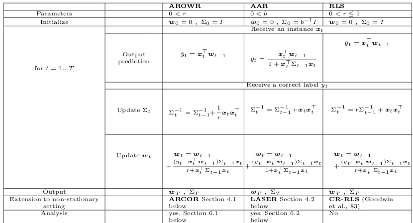
AROWR AAR RLS
Parameters 0< r 0< b 0< r≤1
Initialize w0= 0, Σ0=I w0= 0, Σ0=b−1I w0= 0, Σ0=I
Receive an instancext
fort= 1...T
Output prediction
ˆ
yt=x>twt−1
ˆ yt=
x>twt−1
1 +x>tΣt−1xt
ˆ
yt=x>twt−1
Receive a correct labelyt
Update Σt Σ−t1= Σ−t−11+1 rxtx
>
t Σ
−1
t = Σ
−1
t−1+xtx>t Σ
−1
t =rΣ
−1
t−1+xtx>t
Updatewt wt=wt−1
+(yt−x >
twt−1 )Σt−1xt r+x>tΣt−1xt
wt=wt−1
+(yt−x >
twt−1 )Σt−1xt
1+x>tΣt−1xt
wt=wt−1
+(yt−x >
twt−1 )Σt−1xt r+x>tΣt−1xt
Output wT , ΣT wT , ΣT wT , ΣT
Extension to non-stationary setting
ARCORSection 4.1 below
LASERSection 4.2 below
CR-RLS(Goodwin et al., 83)
Analysis yes, Section 6.1
below
yes, Section 6.2 below
No
Table 1: Algorithms for stationary setting and their extension to non-stationary case
extends AROWR to the non-stationary setting and is similar in spirit to CR-RLS, yet the restart operations it performs depend on the spectral properties of the covariance matrix, rather than the time index t. Additionally, this algorithm performs a projection of the weight vector into a predefined ball. Similar technique was used in first order algorithms by Herbster and Warmuth (2001), and Kivinen and Warmuth (1997). Both steps are motivated from the design and analysis of AROWR. Its design is composed of solving small optimization problems defined in (4), one per input example. The non-stationary version performs explicit corrections to its update, in order to prevent from the covariance matrix to shrink to zero, and the weight-vector to grow too fast.
The second algorithm, described in Section 4.2, is based on a last-step min-max pre-diction principle and objective, where we replace LT(u) in (3) with LT({ut}) and some additional modifications preventing the solution being degenerate. Here the algorithmic modifications from the original AAR algorithm are implicit and are due to the modifica-tions of the objective. The resulting algorithm smoothly interpolates the covariance matrix with the identity matrix.
4.1 ARCOR: Adaptive Regularization of Weights for Regression with Covariance Reset
algorithm uses the update (6) to compute an intermediate candidate for Σt, denoted by
˜ Σt=
Σ−1t−1+1
rxtx
> t
−1
. (7)
If indeed ˜Σt ΛiI then it sets Σt = ˜Σt, otherwise it sets Σt =I and the segment index is increased by 1.
Additionally, before our modification, the norm of the weight vectorwtdid not increase much as the effective learning rate (the matrix Σt) went to zero. After our update, as the learning rate is effectively bounded from below, the norm ofwtmay increase too fast, which in turn will cause a low update-rate in non-stationary inputs.
We thus employ additional modification which is exploited by the analysis. After up-dating the mean wt as in (5),
˜
wt=wt−1+
(yt−x>twt−1)Σt−1xt
r+x>tΣt−1xt
, (8)
we project it into a ballBaround the origin of radiusRBusing a Mahalanobis distance. For-mally, we define the function proj( ˜w,Σ, RB) to be the solution of the following optimization problem
arg min kwk≤RB
1
2(w−w˜) >
Σ−1(w−w˜) .
We write the Lagrangian,
L= 1
2(w−w˜) >
Σ−1(w−w˜) +α
1 2kwk
2−1 2R
2 B
.
Setting the gradient with respect towto zero we get, Σ−1(w−w˜) +αw= 0. Solving for
w we get
w= αI+ Σ−1−1Σ−1w˜ = (I+αΣ)−1w˜ .
From KKT conditions we get that if kw˜k ≤ RB then α = 0 and w = ˜w. Otherwise, α is the unique positive scalar that satisfies k(I+αΣ)−1w˜k = RB. The value of α can be found using binary search and eigen-decomposition of the matrix Σ. We write explicitly Σ =VΛV> for a diagonal matrix Λ. By denoting u=V>w˜ we rewrite the last equation, k(I+αΛ)−1uk = RB. We thus wish to find α such that Pdj u
2 j
(1+αΛj,j)2 = R
2
B. It can be done using a binary search forα∈[0, a] wherea= (kuk/RB−1)/λmin(Λ). To summarize, the projection step can be performed in time cubic indand logarithmic in RB and Λi.
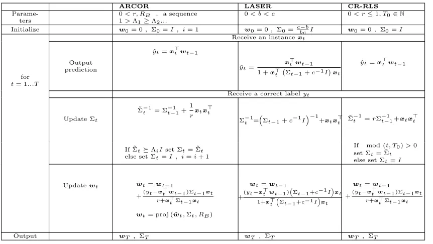
ARCOR LASER CR-RLS
Parame-ters
0< r, RB , a sequence
1>Λ1≥Λ2...
0< b < c 0< r≤1, T0∈N
Initialize w0= 0, Σ0=I , i= 1 w0= 0, Σ0= cbc−bI w0= 0, Σ0=I
Receive an instancext
for t= 1...T
Output prediction
ˆ
yt=x>twt−1
ˆ yt=
x>twt−1
1 +x>t Σt−1+c−1I
xt
ˆ
yt=x>twt−1
Receive a correct labelyt
Update Σt
˜
Σ−t1= Σ−t−11+1 rxtx
>
t
Σ−t1=Σt−1+c−1I
−1
+xtx>t
˜
Σ−t1=rΣt−−11+xtx>t
If ˜ΣtΛiIset Σt= ˜Σt
else set Σt=I , i=i+ 1
If mod (t, T0)>0 set Σt= ˜Σt
else set Σt=I
Updatewt w˜t=wt−1
+(yt−x >
twt−1 )Σt−1xt r+x>tΣt−1xt
wt= proj ( ˜wt,Σt, RB)
wt=wt−1
+(yt−x >
twt−1 )
Σt−1 +c−1I
xt
1+x>t
Σt−1 +c−1I
xt
wt=wt−1
+(yt−x >
twt−1 )Σt−1xt r+x>tΣt−1xt
Output wT , ΣT wT , ΣT wT , ΣT
Table 2: ARCOR, LASER and CR-RLS algorithms
4.2 Last-Step Min-Max Algorithm for Non-Stationary Setting
Our second algorithm is based on a last-step min-max predictor proposed by Forster (1999) and later modified by Moroshko and Crammer (2012) to obtain sub-logarithmic regret in the stationary case. On each round, the algorithm predicts as in the last round, and assumes a worst case choice of yt given the algorithm’s prediction.
We extend the rule given in (3) to the non-stationary setting, and re-define the last-step minmax predictor ˆyT to be1
arg min ˆ yT
max yT
" T X t=1
(yt−yˆt)2− min
u1,..,uT
QT (u1, ...,uT) #
, (9)
where
Qt(u1, . . . ,ut) =bku1k2+c t−1 X s=1
kus+1−usk2+ t X s=1
ys−u>sxs 2
, (10)
for some positive constants b, c. The first term of (9) is the loss suffered by the algorithm whileQt(u1, . . . ,ut) defined in (10) is a sum of the loss suffered by some sequence of linear functions (u1, . . . ,ut), and a penalty for consecutive pairs that are far from each other, and for the norm of the first to be far from zero.
We develop the algorithm by solving the three optimization problems in (9), first, min-imizing the inner term, minu1,..,uTQT(u1, ...,uT), maximizing over yT, and finally, mini-mizing over ˆyT. We start with the inner term for which we define an auxiliary function
Pt(ut) = min
u1,...,ut−1
Qt(u1, . . . ,ut) , which clearly satisfies
min
u1,...,ut
Qt(u1, . . . ,ut) = min
ut
Pt(ut) .
The following lemma states a recursive form of the function-sequence Pt(ut).
Lemma 1 For t= 2,3, . . . P1(u1) =Q1(u1)
Pt(ut) = min
ut−1
Pt−1(ut−1) +ckut−ut−1k2+
yt−u>txt 2
.
The proof appears in Appendix A. Using Lemma 1 we write explicitly the functionPt(ut).
Lemma 2 The following equality holds
Pt(ut) =u>t Dtut−2u>tet+ft ,
where
D1=bI+x1x1> Dt= Dt−1−1 +c
−1
I−1+xtx>t (11)
e1=y1x1 et= I+c−1Dt−1
−1
et−1+ytxt (12)
f1=y21 ft=ft−1−e>t−1(cI +Dt−1)
−1
et−1+y2t . (13) Note thatDt∈Rd×dis a positive definite matrix,et∈Rd×1 andft∈R. The proof appears
in Appendix B. From Lemma 2 we conclude that
min
u1,...,ut
Qt(u1, . . . ,ut) = min
ut
Pt(ut) = min
ut
u>t Dtut−2u>t et+ft
=−e>t Dt−1et+ft .
(14)
Substituting (14) back in (9) we get that the last-step minmax predictor is given by
ˆ
yT = arg min ˆ yT
max yT
" T X t=1
(yt−yˆt)2+e>TD−1T eT −fT #
. (15)
Since eT depends onyT we substitute (12) in the second term of (15),
e>TDT−1eT =
I+c−1DT−1 −1
eT−1+yTxT >
D−1T I+c−1DT−1 −1
eT−1+yTxT
.
Substituting (16) and (13) in (15) and omitting terms not depending explicitly on yT and ˆ
yT we get
ˆ
yT = arg min ˆ yT
max yT
(yT −yˆT)2+yT2x > TD
−1
T xT + 2yTx > TD
−1 T I+c
−1
DT−1 −1
eT−1−y2T
= arg min ˆ yT max yT
x>TDT−1xT
yT2 + 2yT
x>TD−1T I+c−1DT−1 −1
eT−1−yˆT
+ ˆy2T
.
(17)
The last equation is strictly convex in yT and thus the optimal solution is not bounded. To solve it, we follow an approach used by Forster (1999) in a different context. In order to make the optimal value bounded, we assume that the adversary can only choose labels from a bounded set yT ∈ [−Y, Y]. Thus, the optimal solution of (17) over yT is given by the following equation, since the optimal value is yT ∈ {+Y,−Y},
ˆ
yT = arg min ˆ yT
x>TD−1T xT
Y2+ 2Y
x > TD −1 T I+c
−1
DT−1 −1
eT−1−yˆT + ˆy
2 T
.
This problem is of a similar form to the one discussed by Forster (1999), from which we get
the optimal solution, ˆyT =clip
x>TD−1T I+c−1DT−1 −1
eT−1, Y
.
The optimal solution depends explicitly on the bound Y, and as its value is not known, we thus ignore it, and define the output of the algorithm to be
ˆ
yT =x>TD−1T I+c −1D
T−1 −1
eT−1=x>TD−1T D 0
T−1eT−1 , (18)
where we define
D0t−1 = I+c−1Dt−1 −1
. (19)
We call the algorithm LASER for last step adaptive regressor algorithm. Clearly, forc=∞ the LASER algorithm reduces to the AAR algorithm. Similar to CR-RLS and ARCOR, this algorithm can be also expressed in terms of weight-vectorwtand a PSD matrix Σt, by denoting wt=Dt−1et and Σt =D−1t . The algorithm is summarized in the middle column of Table 2.
4.3 Discussion
Table 2 enables us to compare the three algorithms head-to-head. All algorithms perform predictions, and then update the prediction vector wt and the matrix Σt. CR-RLS and ARCOR are more similar to each other, both stem from a stationary algorithm, and perform resets from time-to-time. For CR-RLS it is performed every fixed time steps, while for ARCOR it is performed when the eigenvalues of the matrix (or effective learning rate) are too small. ARCOR also performs a projection step, which is motivated to ensure that the weight-vector will not grow to much, and is used explicitly in the analysis below. Note that CR-RLS (as well as RLS) also uses a forgetting factor (if r <1).
the algorithm implicitly reduces the eigenvalues of the inverse covariance (and increases the eigenvalues of the covariance).
Finally, all three algorithms can be combined with Mercer kernels as they employ only sums of inner- and outer-products of its inputs. This allows them to perform non-linear predictions, similar to SVM.
5. Related Work
There is a large body of research in online learning for regression problems. Almost half a century ago, Widrow and Hoff (1960) developed a variant of the least mean squares (LMS) algorithm for adaptive filtering and noise reduction. The algorithm was further developed and analyzed extensively, for example by Feuer and Weinstein (1985). The normalized least mean squares filter (NLMS) (Bershad, 1986; Bitmead and Anderson, 1980) is similar to LMS but it is insensitive to scaling of the input. The recursive least squares (RLS) (Hayes, 1996) is the closest to our algorithms in the signal processing literature and also maintains a weight-vector and a covariance-like matrix, which is positive semi-definite (PSD), that is used to re-weight inputs.
In the machine learning literature the problem of online regression was studied exten-sively, and clearly we cannot cover all the relevant work. Cesa-Bianchi et al. (1993) studied gradient descent based algorithms for regression with the squared loss. Kivinen and War-muth (1997) proposed various generalizations for general regularization functions. We refer the reader to a comprehensive book in the subject (Cesa-Bianchi and Lugosi, 2006).
Foster (1991) studied an online version of the ridge regression algorithm in the worst-case setting. Vovk (1990) proposed a related algorithm called the Aggregating Algorithm (AA), which was later applied to the problem of linear regression with square loss (Vovk, 1997, 2001). Forster (1999) simplified the regret analysis for this problem. Both algorithms employ second-order information. ARCOR for the separable case is very similar to these algorithms, although has alternative derivation. Recently, few algorithms were proposed either for classification (Cesa-Bianchi et al., 2005; Dredze et al., 2008; Crammer et al., 2008, 2009) or for general loss functions (Duchi et al., 2010; McMahan and Streeter, 2010) in the online convex programming framework. AROWR (Vaits and Crammer, 2011) shares the same design principles of AROW (Crammer et al., 2009) yet it is aimed for regression. The ARCOR algorithm takes AROWR one step further and it has two important modifications which makes it work in the drifting or shifting settings. These modifications make the analysis more complex than of AROW.
Two of the approaches used in previous algorithms for non-stationary setting are bound-ing the weight vector and covariance reset. Boundbound-ing the weight vector was performed either by projecting it into a bounded set (Herbster and Warmuth, 2001), shrinking it by multipli-cation (Kivinen et al., 2001), or subtraction of previously seen examples (Cavallanti et al., 2007). These three methods (or at least most of their variants) can be combined with kernel operators, and in fact, the last two approaches were designed and motivated by kernels.
as far as we know, there is no analysis in the mistake bound model for CR-RLS. Both ARCOR and CR-RLS are motivated from the property that the covariance matrix goes to zero and becomes rank deficient. In both algorithms the information encapsulated in the covariance matrix is lost after restarts. In a rapidly varying environments, like a wireless channel, this loss of memory can be beneficial, as previous contributions to the covariance matrix may have little correlation with the current structure. Recent versions of CR-RLS (Goodhart et al., 1991; Song et al., 2002) employ covariance reset to have numerically stable computations.
ARCOR algorithm combines two techniques with second-order algorithm for regression. In this aspect it has the best of all worlds, fast convergence rate due to the usage of second-order information, and the ability to adapt in non-stationary environments due to projection and resets.
LASER is simpler than all these algorithms as it controls the increase of the eigenvalues of the covariance matrix, implicitly rather than explicitly, by “averaging” it with a fixed di-agonal matrix (see 11), and it does not involve projection steps. The Kalman filter (Kalman, 1960) and the H∞ algorithm (e.g. the work of Simon 2006) designed for filtering take a similar approach, yet the exact algebraic form is different.
The derivation of the LASER algorithm in this work shares similarities with the work of Forster (1999) and the work of Moroshko and Crammer (2012). These algorithms are mo-tivated from the last-step min-max predictor. Yet, the algorithms of Forster and Moroshko and Crammer are designed for the stationary setting, while LASER is primarily designed for the non-stationary setting. Moroshko and Crammer (2012) also discussed a weak variant of the non-stationary setting, where the complexity is measured by the total distance from a reference vector ¯u, rather than the total distance of consecutive vectors (as in this paper), which is more relevant to non-stationary problems.
6. Regret Bounds
We now analyze our algorithms in the non-stationary case, upper bounding the regret using more than a single comparison vector. Specifically, our goal is to prove bounds that would hold uniformly for all inputs, and are of the form
LT(alg)≤LT({ut}) +α(T)
V(P)γ ,
for eitherP = 1 orP = 2, a constantγ and a function α(T) that may depend implicitly on other quantities of the problem.
Specifically, in the next section we show (Corollary 6) that under a particular choice of Λi = Λi(V(1)) for the ARCOR algorithm, its regret is bounded by
LT(ARCOR)≤LT({ut}) +O
T12
V(1) 1 2
logT
.
Additionally, in Section 6.2, we show (Corollary 12) that under proper choice of the constant
c=c V(2)
, the regret of LASER is bounded by
LT(LASER)≤LT({ut}) +O
T23
V(2)
13
The two bounds are not comparable in general. For example, assume a constant instanta-neous driftkut+1−utk=νfor some constant valueν. In this case the variance and squared variance are, V(1) =T ν and V(2) =T ν2. The bound of ARCOR becomes asymptotically
ν12TlogT, while the bound of LASER becomes asymptotically ν 2
3T. Hence the bound of
LASER is better in this case.
Another example is polynomial decay of the drift, kut+1−utk ≤t−κ for some κ >0. In this case, forκ6= 1 we get2 V(1) ≤PTt=1−1t−κ≤RT−1
1 t
−κdt+ 1 = (T−1)1−κ−κ
1−κ . Forκ= 1 we get V(1) ≤ log(T −1) + 1. For LASER we have, for κ 6= 0.5, V(2) ≤ PTt=1−1t−2κ ≤ RT−1
1 t
−2κdt+ 1 = (T−1)1−2κ−2κ
1−2κ . Forκ= 0.5 we getV(2) ≤log(T−1) + 1. Asymptotically, ARCOR outperforms LASER about when κ≥0.7.
Herbster and Warmuth (2001) developed shifting bounds for general gradient descent algorithms with projection of the weight-vector using the Bregman divergence. In their bounds, there is a factor greater than 1 multiplying the term LT ({ut}) (see also theorem 11.4 in Cesa-Bianchi and Lugosi 2006). However, it is possible to get regret bound similar to ARCOR bound above, as they have an implicit parameter that can be tuned with the prior knowledge of LT({ut}) and V(1), leading to regret of O
p
LT({ut})V(1)
, or just
O√T V(1), assuming only the knowledge of V(1).
Busuttil and Kalnishkan (2007) developed a variant of the Aggregating Algorithm (Vovk, 1990) for the non-stationary setting. However, to have sublinear regret they require a strong assumption on the drift V(2) = o(1), while we require only V(2) = o(T) (for LASER) or
V(1) =o(T) (for ARCOR).
6.1 Analysis of the ARCOR Algorithm
Let us define additional notation that we will use in our bounds. We denote by ti the example index for which a restart was performed for the ith time, that is Σti =I for all i.
We define by n the total number of restarts, or intervals. We denote byTi =ti−ti−1 the number of examples between two consecutive restarts. Clearly T = Pni=1Ti. Finally, we denote by Σi−1 = Σti−1 just before theith restart, and we note that it depends on exactly Ti examples (since the last restart).
In what follows we compare the performance of the ARCOR algorithm to the perfor-mance of a sequence of weight vectors ut ∈ Rd, which are of norm bounded by RB. In
other words, all the vectorsutbelong toB. We break the proof into four steps. In the first step (Theorem 3) we bound the regret when the algorithm is executed with some value of parameters {Λi} and the resulting covariance matrices. In the second step, summarized in Corollary 4, we remove the dependencies in the covariance matrices by taking a worst case bound. In the third step, summarized in Lemma 5, we upper bound the total number of switchesn given the parameters {Λi}. Finally, in Corollary 6 we provide the regret bound for a specific choice of the parameters. We now move to state the first theorem.
Theorem 3 Assume that the ARCOR algorithm is run with an input sequence(x1, y1), . . . ,(xT, yT).
Assume that all the inputs are upper bounded by unit norm kxtk ≤1 and that the outputs
are bounded byY = maxt|yt|. Letutbe any sequence of bounded weight vectorskutk ≤RB.
Then, the cumulative loss is bounded by
LT(ARCOR)≤ LT({ut}) + 2RBr X
t 1 Λi(t)
kut−1−utk
+ru>TΣ−1T uT + 2 R2B+Y2
n X
i
log det
Σi−1
,
where nis the number of covariance restarts and Σi−1 is the value of the covariance matrix just before the ith restart.
The proof appears in Appendix C. Note that the number of restarts n is not fixed but depends both on the total number of examplesT and the scheme used to set the values of the lower bound of the eigenvalues Λi. In general, the lower the values of Λiare, the smaller number of covariance-restarts occur, yet the larger the value of the last term of the bound is, which scales inversely proportional to Λi. A more precise statement is given in the next corollary.
Corollary 4 Assume that the ARCOR algorithm made n restarts and {Λi} are monoton-ically decreasing with i (which is satisfied by our choice later). Under the conditions of Theorem 3 we have
LT(ARCOR)≤ LT({ut}) + 2RBrΛ−1n X
t
kut−1−utk
+ 2 R2B+Y2dnlog
1 + T
nrd
+ru>TΣ−1T uT .
Proof By definition we have
Σi−1 =I+1
r
Ti+ti
X t=ti
xtx>t .
Denote the eigenvalues ofPTi+ti
t=ti xtx
>
t byλ1, . . . , λd. Sincekxtk ≤1 their sum is Tr
PTi+ti
t=ti xtx
> t
≤
Ti. We use the concavity of the log function to bound log det
Σi−1=Pd jlog
1 +λj
r
≤
dlog1 +Ti
rd
.We use concavity again to bound the sum
n X
i
log det Σi−1≤ n X
i
dlog
1 + Ti
rd
≤dnlog
1 + T
nrd
,
where we used the fact that Pni Ti =T. Substituting the last inequality in Theorem 3, as well as using the monotonicity of the coefficients, Λi ≥Λn for alli≤n, yields the desired bound.
second term is decreasing with n. If n is small it means that the lower bound Λn is very low (otherwise we would make many restarts) and thus Λ−1n is large. The third term is increasing with nT. We now make this implicit dependence explicit.
Our goal is to bound the number of restartsn as a function of the number of examples
T. This depends on the exact sequence of values Λi used. The following lemma provides a bound onngiven a specific sequence of Λi.
Lemma 5 Assume that the ARCOR algorithm is run with some sequence of Λi. Then, the
number of restarts is upper bounded by
n≤max
N (
N : T ≥r
N X
i
Λ−1i −1 )
.
Proof Since Pn
i=1Ti = T, then the number of restarts is maximized when the number of examples between restarts Ti is minimized. We prove now a lower bound on Ti for all
i= 1. . . n. A restart occurs for the ith time when the smallest eigenvalue of Σt is smaller
(for the first time) than Λi.
As before, by definition, Σi−1 = I + 1rPTi+ti
t=ti xtx
>
t . By a result in matrix analy-sis (Golub and Van Loan, 1996, Theorem 8.1.8) we have that there exists a matrixA∈Rd×Ti
with each column belongs to a bounded convex body that satisfy ak,l ≥0 and Pkak,l ≤1 forl= 1, . . . , Ti, such that thekth eigenvalue λik of Σi−1 equals to λik= 1 + 1rPTi
l=1ak,l. The value ofTi is defined when the largest eigenvalue of Σi
−1
hits Λ−1i . Formally, we get the following lower bound onTi,
arg min {ak,l}
s
s.t. max k 1 +
1
r
s X
l=1
ak,l !
≥Λ−1i
ak,l ≥0 fork= 1, . . . , d, l= 1, . . . , s X
k
ak,l ≤1 forl= 1, . . . , s .
For a fixed value ofs, a maximal value maxk 1 +1rPsl=1ak,l
is obtained when each column of A concentrates the “mass” in one valuek=k0 and equal to its maximal value ak0,l = 1
for l = 1, . . . , s. That is, we have ak,l = 1 for k = k0 and ak,l = 0 otherwise. In this
case maxk 1 +1r Ps
l=1ak,l
= 1 +1rsand the lower bound is obtained when 1 +1rs= Λ−1i . Solving for s we get that the shortest possible length of the ith interval is bounded by,
Ti ≥r Λ−1i −1
. Summing over the last equation we get, T =Pni Ti ≥rPni Λ−1i −1
.
Thus, the number of restarts is upper bounded by the maximal value n that satisfies the last inequality.
withi). This scheme of setting {Λi}balances between the amount of drift (need for many restarts) and the property that using the covariance matrix for updates achieves fast con-vergence. We note that an exponential scheme Λi = 2−i will lead to very few restarts, and very small eigenvalues of the covariance matrix. Intuitively, this is because the last segment will be about half the length of the entire sequence. Combining Lemma 5 with Corollary 4 we get,
Corollary 6 Assume that the ARCOR algorithm is run with a polynomial scheme, that is
Λ−1i =iq−1+ 1for some q >1. Under the conditions of Theorem 3 we have
LT(ARCOR)≤ LT({ut}) +ru>TΣ −1 T uT
+ 2 R2B+Y2d(qT + 1)1q log
1 + T
nrd
(20)
+ 2RBr
(qT + 1)
q−1
q + 1 X
t
kut−1−utk . (21)
Proof Substituting Λ−1i =iq−1+ 1 in Lemma 5 we get
T ≥r
n X
i
Λ−1i −1=r
n X
i=1
iq−1 ≥r
Z n
1
xq−1dx= r
q (n
q−1) ,
where the middle inequality is correct because f(x) = xq−1 for q > 1 is a monotonically increasing function and thus we can upper bound the integral with the right Riemann sum. This yields an upper bound onn,
n≤(qT + 1)1q ⇒ Λ−1
n ≤(qT + 1)
q−1
q + 1.
Comparing the last two terms of the bound of Corollary 6 we observe a natural tradeoff in the value of q. The third term of (20) is decreasing with large values ofq, while the fourth term of (21) is increasing with q.
Assuming a bound on the deviation P
tkut−1 −utk = VT(1) ≤ O T1/p
, or in other words p = (logT)/ logV(1)
. We set a drift dependent parameter q = (2p)/(p+ 1) =
(2 logT)/ logT + logV(1)and get that the sum of (20) and (21) is of orderOT p+1
2p log(T)
=
O√V(1)TlogT.
Few comments are in order. First, as long asp >1 the sum of (20) and (21) iso(T) and thus vanishing. Second, when the drift is very small, that is p ≈ −(1 +), the algorithm sets q ≈ 2 + (2/), and thus it will not make any restarts, and the bound of O(logT) for the stationary case is retrieved. In other words, for this choice ofq the algorithm will have only one interval, and there will be no restarts.
6.2 Analysis of the LASER Algorithm
We now analyze the performance of the LASER algorithm in the worst-case setting in six steps. First, state a technical lemma that is used in the second step (Theorem 8), in which we bound the regret with a quantity proportional to PT
t=1x > t D
−1
t xt. Third, in Lemma 9 we bound each of the summands with two terms, one logarithmic and one linear in the eigenvalues of the matrices Dt. In the fourth (Lemma 10) and fifth (Lemma 11) steps we bound the eigenvalues ofDtfirst for scalars and then extend the results to matrices. Finally, in Corollary 12 we put all these results together and get the desired bound.
Lemma 7 For all t the following statement holds Dt−10 Dt−1xtx>tD−1t D
0
t−1+D0t−1 Dt−1D 0
t−1+c−1I
−Dt−1−1 0 ,
where as defined in (19) we haveD0t−1 = I+c−1Dt−1−1 .
The proof appears in Appendix D. We next bound the cumulative loss of the algorithm.
Theorem 8 Assume that the labels are bounded supt|yt| ≤Y for some Y ∈ R. Then the following bound holds
LT(LASER)≤ min
u1,...,uT
h
LT({ut}) +cVT(2)({ut}) +bku1k2 i
+Y2
T X t=1
x>t Dt−1xt . (22)
Proof Fix t. A long algebraic manipulation, given in Appendix E, yields (yt−yˆt)2+ min
u1,...,ut−1
Qt−1(u1, . . . ,ut−1)− min
u1,...,ut
Qt(u1, . . . ,ut)
= (yt−yˆt)2+ 2ytx>tD −1
t D0t−1et−1+e>t−1 "
−D−1t−1+D0t−1 Dt−1Dt−10 +c−1I
#
et−1
+yt2x>tDt−1xt−yt2 . (23) Substituting the specific value of the predictor ˆyt=x>t D
−1
t Dt−10 et−1from (18), we get that (23) equals to
ˆ
y2t +yt2xt>D−1t xt+e>t−1 "
−Dt−1−1 +Dt−10 D−1t D0t−1+c−1I
#
et−1
= e>t−1D0t−1D−1t xtx>t D −1 t D
0
t−1et−1+y2tx>t Dt−1xt +e>t−1
"
−Dt−1−1 +Dt−10 D−1t D0t−1+c−1I #
et−1
= e>t−1D˜tet−1+y2tx > t D
−1
t xt, (24)
where ˜Dt=Dt−10 Dt−1xtx>tD−1t D0t−1−Dt−1−1 +D0t−1 Dt−1Dt−10 +c−1I
. Using Lemma 7 we upper bound ˜Dt0 and thus (24) is bounded,
Finally, summing overt∈ {1, . . . , T} gives the desired bound,
LT(LASER)− min
u1,...,uT
h
bku1k2+cVT(2)({ut}) +LT({ut}) i
≤Y2
T X t=1
x>t Dt−1xt .
In the next lemma we further bound the right term of (22). This type of bound is based on the usage of the covariance-like matrix D.
Lemma 9
T X t=1
x>tD−1t xt≤ln 1
bDT
+c−1
T X t=1
Tr (Dt−1) . (25)
Proof Let Bt=. Dt−xtx>t = D −1
t−1+c−1I −1
0.
x>t Dt−1xt= Tr
x>tD−1t xt
= TrD−1t xtx>t
= Tr Dt−1(Dt−Bt)
= Tr
D−1/2t (Dt−Bt)D −1/2 t
= TrI−D−1/2t BtD −1/2 t = d X j=1 h
1−λj
Dt−1/2BtD −1/2 t
i
.
We continue using 1−x≤ −ln (x) and get
x>tD−1t xt≤ − d X j=1 ln h λj
Dt−1/2BtD−1/2t i
=−ln d Y j=1 λj
D−1/2t BtDt−1/2
=−ln D
−1/2 t BtD
−1/2 t
= ln|Dt|
|Bt|
= ln |Dt| Dt−xtx>t
.
It follows that
x>t Dt−1xt≤ln
|Dt|
D
−1
t−1+c−1I −1
= ln |Dt|
|Dt−1|
I+c−1Dt−1
= ln |Dt| |Dt−1|
and because ln1bD0
≥0 we get
T X
t=1
x>tD−1t xt≤ln 1
bDT
+ T X t=1
ln I+c−1Dt−1
≤ln 1
bDT
+c−1
T X t=1
Tr (Dt−1) .
At first sight it seems that the right term of (25) may grow super-linearly with T, as each of the matrices Dt grows witht. The next two lemmas show that this is not the case, and in fact, the right term of (25) is not growing too fast, which will allow us to obtain a sub-linear regret bound. Lemma 10 analyzes the properties of the recursion of D defined in (11) for scalars, that isd= 1. In Lemma 11 we extend this analysis to matrices.
Lemma 10 Definef(λ) =λβ/(λ+β) +x2 for β, λ≥0 and some x2 ≤γ2. Then: 1. f(λ)≤β+γ2
2. f(λ)≤λ+γ2
3. f(λ)≤max
λ,3γ2+
√ γ4+4γ2β
2
Proof For the first property we have f(λ) =λβ/(λ+β) +x2 ≤β×1 +x2. The second property follows from the symmetry between β and λ. To prove the third property we decompose the function as, f(λ) = λ− λ2
λ+β +x
2. Therefore, the function is bounded by its argument f(λ) ≤λif, and only if, − λ2
λ+β +x
2 ≤0. Since we assumex2 ≤ γ2, the last inequality holds if,−λ2+γ2λ+γ2β ≤0, which holds for λ≥ γ2+
√ γ4+4γ2β
2 .
To conclude. If λ≥ γ2+ √
γ4+4γ2β
2 , then f(λ) ≤λ. Otherwise, by the second property, we have
f(λ)≤λ+γ2≤ γ 2+p
γ4+ 4γ2β
2 +γ
2= 3γ2+ p
γ4+ 4γ2β
2 ,
as required.
We build on Lemma 10 to bound the maximal eigenvalue of the matricesDt.
Lemma 11 Assume kxtk2 ≤ X2 for some X. Then, the eigenvalues of Dt (for t ≥ 1),
denoted by λi(Dt), are upper bounded by
max
i λi(Dt)≤max (
3X2+√X4+ 4X2c 2 , b+X
2 )
.
with a corresponding eigenvectorvi. From (11) we have
Dt= Dt−1−1 +c−1I −1
+xtx>t
Dt−1−1 +c−1I−1+Ikxtk2 =
d X
i
viv>i
λ−1i +c−1−1+kxtk2
= d X
i
viv>i
λic
λi+c
+kxtk2
. (26)
Plugging Lemma 10 in (26) we get
Dt
d X
i
viv>i max (
3X2+√X4+ 4X2c
2 , b+X 2
)
= max (
3X2+√X4+ 4X2c 2 , b+X
2 )
I .
Finally, equipped with the above lemmas we are able to prove the main result of this section.
Corollary 12 Assume kxtk2 ≤X2, |yt| ≤Y. Then
LT(LASER)≤ bku1k2+LT({ut}) +Y2ln 1
bDT
+c−1Y2Tr (D0) +cV(2)
+c−1Y2T dmax (
3X2+√X4+ 4X2c 2 , b+X
2 )
. (27)
Furthermore, set b= εc for some 0 < ε < 1. Denote by µ = max
9/8X2,(b+X 2)2
8X2
and
M = max3X2, b+X2 . If V(2) ≤T
√ 2Y2dX
µ3/2 (low drift) then by setting
c=
√
2T Y2dX
V(2)2/3 (28)
we have
LT(LASER)≤ bku1k2+ 3 √
2Y2dX2/3T2/3V(2)1/3+ ε 1−εY
2d+L
T({ut})
+Y2ln 1
bDT
The proof appears in Appendix F. Note that if V(2) ≥ TY2µdM2 then by setting c =
p
Y2dM T /V(2) we have
LT(LASER)≤bku1k2+ 2 p
Y2dT M V(2)+ ε
1−εY
2d+L
T({ut}) +Y2ln 1
bDT
. (30)
(see Appendix G for details). The last bound is linear inT and can be obtained also by a naive algorithm that outputs ˆyt= 0 for allt.
A few remarks are in order. When the variance V(2) = 0 goes to zero, we set c = ∞ and thus we have Dt = bI +Pts=1xsx>s used in recent algorithms (Vovk, 2001; Forster, 1999; Hayes, 1996; Cesa-Bianchi et al., 2005). In this case the algorithm reduces to the algorithm by Forster (1999) (which is also the AAR algorithm of Vovk 2001), with the same logarithmic regret bound (note that the term ln1bDT
in the bounds is logarithmic in T, see the proof of Forster 1999). See also the work of Azoury and Warmuth (2001).
7. Simulations
We evaluated our algorithms on four data sets, one synthetic and three real-world. The synthetic data set contains 2,000 points xt ∈ R20, where the first ten coordinates were
grouped into five groups of size two. Each such pair was drawn from a 45◦ rotated Gaussian distribution with standard deviations 10 and 1. The remaining 10 coordinates of xt were drawn from independent Gaussian distributionsN (0,2). The data set was generated using a sequence of vectors ut ∈ R20 for which the only non-zero coordinates are the first two,
where their values are the coordinates of a unit vector that is rotating with a constant rate. Specifically, we have kutk = 1 and the instantaneous drift kut−ut−1k is constant. The labels were set according toyt=x>t ut.
The first two real-world data sets were generated from echoed speech signal. The first speech echoed signal was generated using FIR filter with k delays and varying attenuated amplitude. This effect imitates acoustic echo reflections from large, distant and dynamic obstacles. The difference equation y(n) = x(n) +PkD=1A(n)x(n−D) +v(n) was used, whereDis a delay in samples, the coefficientA(n) describes the changing attenuation related to object reflection andv(n)∼ N 0,10−3is a white noise. The second speech echoed signal was generated using a flange IIR filter, where the delay is not constant, but changing with time. This effect imitates time stretching of audio signal caused by moving and changing objects in the room. The difference equationy(n) =x(n) +Ay(n−D(n)) +v(n) was used. The last real-world data set was taken from the Kaggle competition ”Global Energy Forecasting Competition 2012 - Load Forecasting”.3 This data set includes hourly demand for four and a half years from 20 different geographic regions, and similar hourly temperature readings from 11 zones, which we used as features xt ∈ R11. Based on this data set, we
generated drifting and shifting data as follows: we predict the load 3 times a day (thus there is a drift between day and night), and every half a year there is a switch in the region where the load is predicted.
Five algorithms were evaluated: NLMS (normalized least mean square) (Bershad, 1986; Bitmead and Anderson, 1980) which is a state-of-the-art first-order algorithm, AROWR
3. The data set was taken from
200 400 600 800 1000 1200 1400 1600 1800 2000 20
40 60 80 100 120 140 160
Iteration
Cumultive Square−Error
synthetic data
CR RLS ARCOR NLMS AROW LASER
(a)
0.5 1 1.5 2 2.5 3 3.5 x 10⁴ 10
20 30 40 50 60 70 80
Iteration
Cumultive Square−Error
speech signal with echo CR RLS
ARCOR NLMS AROW LASER
(b)
0.5 1 1.5 2 2.5 3 3.5 x 10⁴ 20
40 60 80 100 120 140
Iteration
Cumultive Square−Error
speech signal with additive echo CR RLS
ARCOR NLMS AROW LASER
(c)
0 500 1000 1500 2000 2500 3000 3500 4000 0
50 100 150 200 250 300 350 400 450 500
Iteration
Cumultive Square−Error
electric load data
CR RLS ARCOR NLMS AROW LASER
(d)
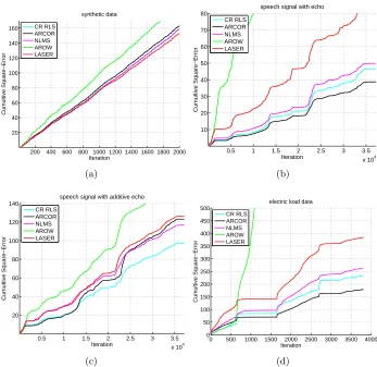
Figure 1: Cumulative squared loss for AROWR, ARCOR, LASER, NLMS and CR-RLS vs iteration. (a) Results for synthetic data set with drift. (b) Results for a problem of acoustic echo cancellation on speech signal generated using FIR filter and (c) IIR filter. (d) Results for a problem of electric load prediction (best shown in color).
The results are summarized in Figure 1. AROWR performs the worst on all data sets as it converges very fast and thus not able to track the changes in the data. Focusing on Figure 1(a), showing the results for the synthetic signal, we observe that ARCOR performs relatively bad as suggested by our analysis for constant, yet not too large, drift. Both CR-RLS and NLMS perform better, where CR-RLS is slightly better as it is a second-order algorithm, and allows to converge faster between switches. On the other hand, NLMS is not converging and is able to adapt to the drift. Finally, LASER performs the best, as hinted by its analysis, for which the bound is lower where there is a constant drift.
Moving to Figure 1(b), showing the results for first echoed speech signal with varying amplitude, we observe that LASER is the worst among all algorithms except AROWR. Indeed, it prevents the convergence by keeping the learning rate far from zero, yet it is a min-max algorithm designed for the worst-case, which is not the case for real-world speech data. However, speech data is highly regular and the instantaneous drift vary. NLMS performs better as it does not converge, yet both CR-RLS and ARCOR perform even better, as they both do not converge due to covariance resets on the one hand, and second-order updates on the other hand. ARCOR outperforms CR-RLS as the former adapts the resets to actual data, and does not use pre-defined scheduling as the later.
Figure 1(c) summarizes the results for evaluations on the second echoed speech signal. Note that the amount of drift grows since the data is generated using flange filter. Both LASER and ARCOR are outperformed as both assume drift that is sublinear or at most linear, which is not the case. CR-RLS outperforms NLMS. The later is first order, so is able to adapt to changes, yet has slower convergence rate. The former is able to cope with drift due to resets.
Finally, Figure 1(d) summarizes the results for the electric load data set. ARCOR outperforms other algorithms, as the drift is sublinear and it has the ability to adapt resets to the data. Again, LASER is a min-max algorithm designed for the worst case, which is usually not the case for real-world data.
Interestingly, in all experiments, NLMS was not performing the best nor the worst. There is no clear winner among the three algorithms that are both second-order (AR-COR, LASER, CR-RLS), and designed to adapt to drifts. Intuitively, if the drift suits the assumptions of an algorithm, that algorithm would perform the best, and otherwise, its performance may even be worse than of NLMS.
0.5 1 1.5 2 2.5 3 3.5 x 10⁴ 5
10 15 20 25 30 35 40 45 50 55
Iteration
Cumultive Square−Error
speech signal with echo
ARCOR − no proj, poly ARCOR − proj, poly ARCOR − no proj, const ARCOR − proj, const
0.5 1 1.5 2 2.5 3 3.5 x 10⁴ 20
40 60 80 100 120 140
Iteration
Cumultive Square−Error
speech signal with additive echo
ARCOR − no proj, poly ARCOR − proj, poly ARCOR − no proj, const ARCOR − proj, const
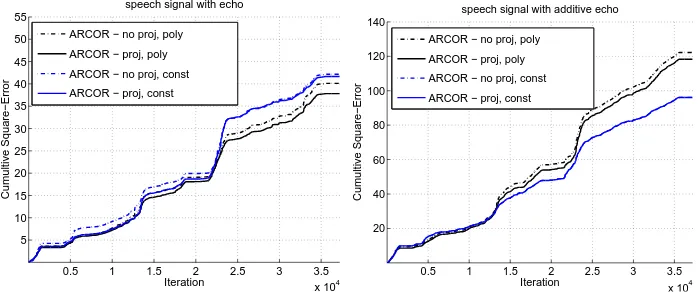
Figure 2: Cumulative squared loss of four variants of ARCOR vs iteration.
and performs the best in this case. However, when this assumption over the amount of drift breaks, this version is not optimal anymore, and constant scheme performs better, as it allows the algorithm to adapt to non-vanishing drift. Finally, in both data sets, the algorithm that performs the best performs a projection step after each iteration, providing some empirical evidence for its need.
8. Summary and Conclusions
We proposed and analyzed two novel algorithms for non-stationary online regression de-signed and analyzed with the squared loss in the worst-case regret framework. The AR-COR algorithm was built on AROWR. It employs second-order information, yet performs data-dependent covariance resets, which provides it the ability to track drifts. The LASER algorithm was built on the last-step minmax predictor with the proper modifications for non-stationary problems. Our algorithms require some prior knowledge of the drift to get optimal performance, and each algorithm works best in other drift level. The optimal set-ting depends on the actual drift in the data and the optimality of our bounds is an open issue.
Few open directions are possible. First, extension of these algorithms to other loss functions rather than the squared loss. Second, currently, direct implementation of both algorithms requires either matrix inversion or eigenvector decomposition. A possible direc-tion is to design a more efficient version of these algorithms. Third, an interesting direcdirec-tion is to design algorithms that automatically detect the level of drift, or do not need this information before run-time.
Appendix A. Proof of Lemma 1
Proof We calculate
Pt(ut) = min
u1,...,ut−1
bku1k2+c t−1 X s=1
kus+1−usk2+ t X s=1
ys−u>sxs 2!
= min
u1,...,ut−1
bku1k2+c t−2 X s=1
kus+1−usk2+ t−1 X s=1
ys−u>sxs 2
+ckut−ut−1k2
+yt−u>txt 2!
= min
ut−1
min
u1,...,ut−2
bku1k2+c t−2 X s=1
kus+1−usk2+ t−1 X s=1
ys−u>sxs 2
+ckut−ut−1k2
+
yt−u>txt 2!
= min
ut−1
" min
u1,...,ut−2
bku1k2+c t−2 X s=1
kus+1−usk2+ t−1 X s=1
ys−u>sxs 2
+ckut−ut−1k2+
yt−u>t xt 2#
= min
ut−1
Pt−1(ut−1) +ckut−ut−1k2+
yt−u>t xt 2!
.
Appendix B. Proof of Lemma 2
Proof By definition
P1(u1) =Q1(u1) =bku1k2+
y1−u>1x1 2
=u>1 bI+x1x>1
u1−2y1u>1x1+y12 ,
We proceed by induction, assume that,Pt−1(ut−1) =u>t−1Dt−1ut−1−2u>t−1et−1+ft−1. Applying Lemma 1 we get
Pt(ut) = min
ut−1
u>t−1Dt−1ut−1−2u>t−1et−1+ft−1+ckut−ut−1k2+
yt−u>t xt 2!
= min
ut−1
u>t−1(cI+Dt−1)ut−1−2u>t−1(cut+et−1) +ft−1+ckutk2
+yt−u>t xt 2!
=−(cut+et−1)>(cI +Dt−1)−1(cut+et−1) +ft−1+ckutk2+
yt−u>txt 2
=u>t cI+xtxt>−c2(cI+Dt−1)−1
ut−2u>t h
c(cI+Dt−1)−1et−1+ytxt i
−e>t−1(cI+Dt−1)−1et−1+ft−1+y2t .
Using the Woodbury identity we continue to develop the last equation,
=u>t cI+xtx>t −c2 h
c−1I −c−2 Dt−1−1 +c−1I−1iut
−2u>t
h
I+c−1Dt−1 −1
et−1+ytxt i
−e>t−1(cI+Dt−1) −1
et−1+ft−1+y2t =u>t
D−1t−1+c−1I−1+xtx>t
ut−2u>t h
I+c−1Dt−1 −1
et−1+ytxt i
−e>t−1(cI+Dt−1)−1et−1+ft−1+y2t , and indeed Dt = D−1t−1+c−1I
−1
+xtx>t , et = I+c−1Dt−1 −1
et−1 +ytxt and, ft =
ft−1−e>t−1(cI+Dt−1)−1et−1+y2t, as desired.
Appendix C. Proof of Theorem 3
We prove the theorem in four steps. First, we state a technical lemma, for which we define the following notation
dt(z,v) = (z−v)>Σ−1t (z−v),
d˜t(z,v) = (z−v) >Σ˜−1
t (z−v),
χt=x>t Σt−1xt .
Lemma 13 Let w˜t and Σ˜t be defined in (7)and (8), then
dt−1(wt−1,ut−1)−d˜t( ˜wt,ut−1) = 1
r`t−
1
rgt−
`tχt
r(r+χt)
,
where `t= yt−w>t−1xt 2
and gt= yt−u>t−1xt 2
.
Proof We start by writing the distances explicitly,
dt−1(wt−1,ut−1)−d˜t( ˜wt,ut−1)
=−(ut−1−w˜t)>Σ˜−1t (ut−1−w˜t) + (ut−1−wt−1)>Σ−1t−1(ut−1−wt−1) .
Substituting ˜wt as appears in (8) the last equation becomes
−(ut−1−wt−1)>Σ˜−1t (ut−1−wt−1) + 2(ut−1−wt−1) ˜Σ−1t Σt−1xt
(yt−x>twt−1)
r+x>t Σt−1xt
−
(yt−x>t wt−1)
r+x>t Σt−1xt 2
x>t Σt−1Σ˜−1t Σt−1xt+ (ut−1−wt−1)>Σ−1t−1(ut−1−wt−1) .
Plugging ˜Σt as appears in (7) we get
dt−1(wt−1,ut−1)−d˜t( ˜wt,ut−1) =−(ut−1−wt−1)>
Σ−1t−1+1
rxtx
> t
(ut−1−wt−1)
+ 2(ut−1−wt−1)>
Σ−1t−1+1
rxtx
> t
Σt−1xt
(yt−x>t wt−1)
r+x>t Σt−1xt
− (yt−x > twt−1)2
r+x>t Σt−1xt 2x
> t Σt−1
Σ−1t−1+1
rxtx
> t
Σt−1xt
Finally, we substitute `t = yt−xt>wt−12 , gt = yt−x>t ut−12 and χt = x>t Σt−1xt. Rearranging the terms,
dt−1(wt−1,ut−1)−d˜t( ˜wt,ut−1) =−1
r
yt−x>twt−1−
yt−x>t ut−1 2
−2 yt−x >
tut−1− yt−x>twt−1
yt−x>t wt−1
r+χt
1 +χt
r
− `tχt (r+χt)2
1 +χt
r
=−1
r`t+ 2
yt−x>t wt−1 yt−x>tut−1 1
r −
1
rgt
+ 2`t
r+χt
1 +χt
r
− `tχt
r(r+χt)
−2 yt−x >
t wt−1 yt−x>t ut−1
r+χt
1 +χt
r
=1
r`t−
1
rgt−
`tχt
r(r+χt)
,
which completes the proof.
We now define one element of the telescopic sum and lower bound it.
Lemma 14 Denote
∆t=dt−1(wt−1,ut−1)−dt(wt,ut)
then
∆t≥ 1
r (`t−gt)−`t χt
r(r+χt)
+u>t−1Σ−1t−1ut−1−u>tΣ−1t ut−2RBΛ−1i kut−1−utk ,
where i−1 is the number of restarts occurring before example t.
Proof We write ∆t as a telescopic sum of four terms as follows ∆t,1=dt−1(wt−1,ut−1)−d˜t( ˜wt,ut−1) ∆t,2=d˜t( ˜wt,ut−1)−dt( ˜wt,ut−1) ∆t,3=dt( ˜wt,ut−1)−dt(wt,ut−1)
∆t,4=dt(wt,ut−1)−dt(wt,ut) .
We lower bound each of the four terms. Since the value of ∆t,1was computed in Lemma 13, we start with the second term. If no reset occurs then Σt= ˜Σt and ∆t,2 = 0. Otherwise, we use the facts that 0Σ˜tI and Σt=I, and get
∆t,2= ( ˜wt−ut−1)>Σ˜−1t ( ˜wt−ut−1)−( ˜wt−ut−1)>Σ−1t ( ˜wt−ut−1)
≥Tr( ˜wt−ut−1) ( ˜wt−ut−1)>(I−I)
To summarize, ∆t,2 ≥ 0. We can lower bound ∆t,3 ≥ 0 by using the fact that wt is a projection of ˜wt onto a closed set (a ball of radius RB around the origin), which by our assumption contains ut. Employing Corollary 3 of Herbster and Warmuth (2001) we get,
dt( ˜wt,ut−1)≥dt(wt,ut−1) and thus ∆t,3 ≥0. Finally, we lower bound the fourth term ∆t,4,
∆t,4= (wt−ut−1)>Σ−1t (wt−ut−1)−(wt−ut)>Σ−1t (wt−ut) =u>t−1Σ−1t ut−1−u>t Σ
−1
t ut−2w>t Σ −1
t (ut−1−ut) . (31)
We use the H¨older inequality and then the Cauchy-Schwartz inequality to get the following lower bound
−2w>tΣ−1t (ut−1−ut) =−2Tr
Σ−1t (ut−1−ut)w>t
≥ −2λmax Σ−1t
w>t (ut−1−ut) ≥ −2λmax Σ−1t
kwtkkut−1−utk .
Using the facts that kwtk ≤RB and that λmax Σ−1t
= 1/λmin(Σt)≤Λ−1i , where iis the current segment index, we get
−2w>t Σ−1t (ut−1−ut)≥ −2Λ−1i RBkut−1−utk . (32)
Substituting (32) in (31) and using ΣtΣt−1 a lower bound is obtained,
∆t,4 ≥u>t−1Σ−1t ut−1−u >
tΣ−1t ut−2RBΛ−1i kut−1−utk
≥u>t−1Σ−1t−1ut−1−u>t Σ−1t ut−2RBΛ−1i kut−1−utk . (33)
Combining (33) with Lemma 13 concludes the proof.
Next we state an upper bound that will appear in one of the summands of the telescopic sum.
Lemma 15 During the runtime of the ARCOR algorithm we have
ti+Ti
X t=ti
χt (χt+r)
≤logdetΣ−1t
i+1−1
= logdet Σi−1.
We remind the reader that ti is the first example index after the ith restart, and Ti is the
number of examples observed before the next restart. We also remind the reader the notation
Σi= Σti+1−1 is the covariance matrix just before the next restart.
The proof of the lemma is similar to the proof of Lemma 4 by Crammer et al. (2009) and thus omitted. We now put all the pieces together and prove Theorem 3.
Proof We bound the sumP
t∆t from above and below, and start with an upper bound using the property of telescopic sum,
X t
∆t= X
t