INTEGRATED WATER RESOURCES
MANAGEMENT
LAND USE DYNAMICS AND BIODIVERSITY
ENERGY EFFICIENCY AND RENEWABLE
RESOURCES
REGIONAL MANAGEMENT AND
SUSTAINABLE LIVELIHOODS OF THE POOR
VOLUME 7 - 2017
DOI: 10.5027/jnrd.v7i0.01 - DOI: 10.5027/jnrd.v7i0.12
Multi-Level Land Cover Change Analysis in the Forest-Savannah Transition Zone of the Kintampo Municipality, Ghana 1 Authors: Raymond Aabeyir, Wilson Agyei Agyare, Michael J. C. Weir and Stephen Adu-Bredu
DOI: 10.5027/jnrd.v7i0.01
Condition, Tendency, and Dynamic Interactions in a Resilience Context of a Social-Ecological System 12 Authors: Carolin Antoni, Elisabeth Huber-Sannwald, Humberto Reyes Hernández and Anuschka van´t Hooft
DOI: 10.5027/jnrd.v7i0.02
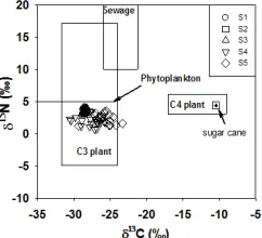
Tracing Anthropogenic Disturbances of a Wetland Through Carbon and Nitrogen Isotope Analyses in Sediments 22 Authors: F. Virginia Pérez-Castillo, M. Catalina Alfaro-De la Torre, Rebeca Y. Pérez-Rodriguez and Francisco A. Comín Sebastián
DOI: 10.5027/jnrd.v7i0.03
Implementation of Fuzzy Sets in the Non-Isothermal Pyrolysis of Biomass 30
Authors: Alok Dhaundiyal and Suraj B. Singh DOI: 10.5027/jnrd.v7i0.04
Land Use/Land Cover Factor Values and Accuracy Assessment Using a GIS and Remote Sensing in the Case of the Quashay
Wa-tershed in Northwestern Ethiopia 38
Authors: Habtamu Tadele, Asnake Mekuriaw, Yihenew G. Selassie and Lewoye Tsegaye DOI: 10.5027/jnrd.v7i0.05
Combination of MODIS Vegetation Indices, GRACE Terrestrial Water Storage Changes, and In-Situ Measurements for Drought
Assessment in Cagayan River Basin, Philippines 45
Author: Anjillyn Mae C. Perez and Ariel C. Blanco DOI: 10.5027/jnrd.v7i0.06
Impact of Urbanization and Climate Change on Urban Flooding: A case of the Kathmandu Valley 56 Authors: Inu Pradhan-Salike and Jiba Raj Pokharel
DOI: 10.5027/jnrd.v7i0.07
Profile Characteristics of Watershed Farmers and the Extent of Adoption of NRM Practices in Watershed Areas of the Andhra
Pra-desh State 67
Authors: Archana Palle, M. Jagan Mohan Reddy and I. Sreenivasa Rao DOI: 10.5027/jnrd.v7i0.08
The Role of Trust-building in Fostering Cooperation in the Eastern Nile Basin: A Case of Experimental Game Application 73 Author: Mahsa Motlagh, Anik Bhaduri, Janos J. Bogardi and Lars Ribbe
DOI: 10.5027/jnrd.v7i0.09
Participation of Urban Women in Agricultural Production Activities in the Sokoto Metropolis, Nigeria 84 Author: Barau, A. A. and Oladeji, D. O.
DOI: 10.5027/jnrd.v7i0.10
Capacity of Albit® Plant Growth Stimulator for Mitigating Side-effects of Pesticides on Soil Microbial Respiration 91
Authors: Natalia N. Karpun, Eleonora B. Yanushevskaya, Yelena V. Mikhailova, Pedro Mondaca and Alexander Neaman DOI: 10.5027/jnrd.v7i0.11
Adaptive Thermal Comfort in Learning Spaces: A Study of the Cold Period in Ensenada, Baja California 96 Authors: Julio Rincón, Gonzalo Bojórquez, Víctor Fuentes and Claudia Calderón
JOURNAL OF
NATURAL RESOURCES
AND DEVELOPMENT
Multi-Level Land Cover Change Analysis in the
Forest-Savannah Transition Zone of the Kintampo
Municipality, Ghana
Raymond Aabeyir
ab*, Wilson Agyei Agyare
c, Michael J. C. Weir
dand Stephen Adu-Bredu
e a WASCAL Graduate Research Programme, on Climate Change and Land Use, KNUSTb Department of Environment and Resource Studies, UDS-Wa Campus, Ghana c Department of Agricultural Engineering, KNUST, Kumasi, Ghana
d Department of Natural Resources, Faculty of Geoinformation Science and Earth Observation (ITC), University of Twente, the Netherlands e Biodiversity Conservation and Ecosystem Services Division, Forestry Research Institute of Ghana, Kumasi, Ghana
*Corresponding author: [email protected] [email protected]
Abstract
Received 27/02/2017 Accepted 23/05/2017 Published 31/05/2017
Article history
Change detection Multi-level analysis Land cover Forest-Savannah Ghana
Keywords
This study presents a multi-level analysis of land cover change in the Kintampo Municipality of Ghana using Landsat TM, ETM + and Landsat 8 images from 1986, 2001 and 2014, respectively. The expected and observed annual rates of land cover change for the periods 1986 to 2001 and 2001
to 2014 were analyzed at temporal and intra and inter-land cover levels using post-classification
change detection. The results reveal that the expected annual rate of land cover change for the time intervals is 2.55 %. The observed annual rate of change from 2001 to 2014 is 2.63 %, which is greater than the expected value. This shows that land cover changed faster than expected in this period. The observed intra-land cover gains and losses for woodland is 2.49 % which is less than expected for the change periods. This suggests that the observed gain and loss in woodlands are attributable to random changes. The inter-land cover level changes for both periods reveal that when woodland gained or lost, it did not target shrub/grassland. This shows that the process of gain or loss in woodland in both periods was random. This is an indication that woodland cover is sustained by
a slow, natural regeneration process and not by anthropogenic activities. The findings highlight the
Land cover change arises from both natural and anthropogenic causes. In general, the former is progressive and gradual while the latter is often rapid and sudden due to increasing population pressure [1], [2]. Anthropogenic land cover change poses a threat to the global natural environment because of the rapid nature of how it occurs, thus making it the most prominent form of global environmental change occurring at both a spatial and a temporal scale [3]. Anthropogenic land cover change is often a reflection of the most significant impact of human activities on the environment,
especially in fragile ecosystems [4], [5][6].
The current pace, magnitude and spatial extent of land cover change
are unprecedented and significantly affect key aspects of Earth System
functioning, notably climate change and ecosystem services [7], [8] [9]. It has been observed that about one third of the earth surface
is affected by human modifications [10], [11] and the modifications
are still on-going as population and the resulting demand for land continue to increase [12]. On-going anthropogenic land cover change occurs at a rate of 13 million ha year-1, with serious consequences for climate change [11]. Consequently, the analysis of land cover changes at global, regional, national and local levels is viewed as a critical step to policy decisions on climate change, adaptation and mitigation activities. Despite the critical role land cover analysis plays, many land cover change analyses ([6], [13]–[18]) have focused
on the identification of patterns of change and simple quantities of
change, which often leads to a simplistic understanding of land cover dynamics [19], [20]. Such land cover change analyses normally fail to highlight temporal, intra and inter-land cover changes, which are relevant for policy makers as they indicate the nature and direction of the change among land cover types, and whether the land cover change is driven by a systematic or a random process [19]–[22], [21].
The direction of land cover change must be identified before any
causal relationship can be postulated [23].
The objective of this study is to assess the temporal, intra and inter-land cover transitions in the Kintampo Municipality of Ghana for the period between 1986 and 2014. The Municipality is known for commercial charcoal production and farming in Ghana [24]. Woodland degradation in the Municipality is largely attributed to commercial charcoal production and farming [24]. Therefore, increasing charcoal production and farming activities is currently exerting undue pressure on the already stressed woodlands [25]. As observed in a similar charcoal producing and farming community, charcoal production and farming have dictated and continue to dictate the state of land cover due to economic desperation and a need to meet immediate income needs [26]. This raises questions about changes in land cover over time in the municipality.
Thus, assessment of temporal, intra and inter-land cover change is relevant for identifying the interval within which these changes are fast, the land cover types that are gaining or losing more than what is expected under a random process of change, the sources and destinations of the gains and losses in each land cover type and
whether the losses are random or systematic. This information is critical to decision makers to ensure that policies are formulated to target systematic processes of land cover change and not random processes. Furthermore, understanding each level of transition is important for climate change mitigation programs, such as Reducing Emissions from Deforestation and forest Degradation coupled with enhancing existing carbon stock (REDD+) [27], [28]. For instance, the UNFCCC is yet to specify exactly what land-use reforms and activities will be promoted and rewarded under a future REDD+ mechanism. Taking such decisions depends on the availability of information from land cover assessments [29].
2.1 Description of the study area
The study was conducted in the Kintampo Municipality of the Brong-Ahafo Region, Ghana. The municipality lies between latitudes 7º 45’ N and 8º 50’ N and longitudes 1º 0’ W and 2º 15’ W (Figure 1) with a total surface area of about 5,108 km². It shares boundaries with the Central Gonja District to the North; the Bole District to the West; the East Gonja District to the North-East; the Kintampo South District to the South; and the Pru District to the South-East. The mean annual rainfall is between 1000 mm and 1200 mm and occurs in two seasons; May to August as the major rainy season and September to October as the minor rainy season [30]. The mean monthly temperature ranges from 30° C in March to 24° C in August, with a relative humidity varying from 90 % to 95 % in the rainy seasons and 75 % to 80 % in the dry season. The Municipality is part of the Forest-Savannah transition zone of Ghana, located between the Forest ecological zone in the south and the Savannah ecological zone in the north of the country [31], [32], [4]. However, the vegetation has more savannah-like characteristics compared to forest characteristics because it has lost most of its original forest cover due to anthropogenic activities
[31], [4]. Kintampo Municipality has a total population of 95,480 with a growth rate of 2.6 % [32]. The Municipality is a net receiver of immigrants, mainly settler farmers and charcoal producers [33]. Farming and charcoal production are major economic activities in the rural communities of the municipality [25]. About 71.1 % of the total working population is employed in agriculture and charcoal production and 28.9 % in commerce, industry and services [33]. The study site within the municipality was selected on the basis that Kintampo, the municipal capital, is expanding at a fast rate to accommodate the increasing number of immigrants. Furthermore, Asantekwa, Kunsu, Babatokuma, Attakura and Dawadawa are major farming and charcoal producing communities. Expansion of the municipality, and the increasing expansion of farmlands and charcoal
production influence the dynamics of the vegetation cover of the area at different levels (temporal, intra and inter-land cover), hence
the need to conduct a multi-level land cover assessment of the area.
2.2 Description of Images and Software
Landsat TM, ETM + and Landsat 8 images from 1986, 2001 and
1. Introduction
2014, respectively, were used for the study based on a combination of the following considerations: cost of acquiring alternative high resolution images, availability of images covering the study area, appropriateness of the spatial resolution and temporal interval for change detection analysis [34]. Long time periods such as 10 – 11 years are often best for describing long-term changes such as woodland degradation due to logging and woodland recovery [34]. Charcoal production and farming being major drivers of land cover change in the Kintampo Municipality, an interval of 10 years was considered appropriate for this study. However, due to unavailability of cloud-free satellite images of the study area, it was not possible to use a ten-year time interval. The same limitation also resulted in the
unequal time interval for the two periods. The difference in the time
interval was accounted for by normalizing the extent of the changes in land cover. They were downloaded with path 194 and row 054 from the Global Land Cover Facility (GLCF) website. The 1986, 2001 and 2014 scenes were captured in the dry season on 11th November 1986, 12th January 2001 and 26th December 2014, respectively. The Landsat TM and ETM+ images are cloud free while the Landsat 8 image has 0.14 % cloud cover, which extends to a portion of the study area (Figure 1). Color Infrared band combinations of Red, Green and Blue (RGB) were used. Band combinations of 432 for Landsat TM and 543 for ETM+ and Landsat 8 were used for the image composite. These band combinations discriminate vegetation well [4]. Google Earth images, WorldView-2 images acquired on 12th January 2014, 14th February 2011, 2nd April 2015 and 6th April 2012 and Quickbird images acquired on 13th March 2012 from DigitalGlobe Foundation
were used to validate the resulting classified images from 1986 and
2001. Remote Sensing software was used to process and classify the images and perform the change detection, and Geographic Information System (GIS) software was used to process and add map
properties to the classified and changed images.
2.3 Image Processing
Radiometric correction was performed to remove any inconsistency between spectral values captured by sensors and the spectral radiation brightness of the objects [35]. Misregistration can affect the
accuracy of change detection results substantially. A misregistration of less than 0.2 pixel size is required to achieve a change detection error of less than 10 % [36]. The images were already geo-referenced to Universal Transverse Mercator (UTM) Zone 30 N. However, this geo-referencing was validated to check the geometric accuracies of the images. For this purpose, coordinates of well distributed 30
Ground Control Points (GCP), which were identifiable on the 2014
image, recorded with Garmin hand-held Global Positioning System (GPS) receiver (GPSmap 62s, Garmin, USA) were used. Of the 30
GCPs, 21 and 24 were identifiable on the 2001 and 1986 images,
respectively. The extracted GCPs were road intersections, sharp curves and bridges across major rivers [22]. The Root Mean Square Error (RMSE) was computed using (Equation 1) [37]:
(1)
where (X, Y) and (x, y) are ground and image coordinates respectively and n is the number of reference points.
Generally, it is recommended that the RMSE of a good registration should be less than half a pixel [22], [38]. However, Dai & Khorram
[36] observed that for purposes of change detection, a registration accuracy of less than 0.2 pixel is generally required to detect 90 % of true change. The computed RMSE values were ± 5.1 m, 5.3 and ± 5.7 m for 2014, 1986 and 2001 images, respectively, which are less than 0.2 pixel size of the images used (30 m × 30 m Landsat image).
2.4 Description of land cover types
Three land cover classes, namely woodland, shrub/grassland, bare
land/settlement were identified for the purpose of this study. Each
of these classes is described in Table 1. Although it would have been desirable to separate grass land from shrub/fallow land, and bare land from settlement, farmlands and home gardens, this was
not possible due the difficulty in separating them in the preliminary classification processes. This is because the images were captured in
the dry season during which farmlands, home gardens and bare land appear similar, while fallow lands, shrub and grass also look similar. However, the three classes served the purpose of the study since the primary objective of the land cover assessment was to understand the transition of woodland to non-woodland.
Figure 1: Kintampo Municipality. Adapted from [30]
2.5 Image Classification
Supervised classification was performed using Gaussian Maximum Likelihood Classifier (MLC) for the 2014 (Landsat 8) image. The MLC
was trained with 100 land cover samples. One hundred and twenty (120) homogeneous pixels per land cover sample were selected on the image and assigned the appropriate class name. The MLC
classifies an unknown pixel by computing and evaluating its probability of belonging to each land cover class defined during the
training process and then assigns the pixel to the class for which it has the highest probability [42]. The MLC was chosen based on its advantages [43], [44]. It quantitatively evaluates both the variance and correlation of a category of spectral response patterns when classifying an unknown pixel [45], [43]. Atmospheric correction has
little effect on the accuracy of a single date image classification using
MLC provided both the image and training data are on the same relative scale (either corrected or uncorrected) [44]. Despite the advantages of MLC, its application requires that pixel values of the image and training samples are normally distributed. MLC provides
good classification results of multispectral data, since it takes into
account the shape, size and orientation of a cluster [43] in assigning an unknown pixel to a cluster.
A statistical unsupervised clustering algorithm, the Iterative Self-Organizing Data Analysis Technique (ISODATA) [46], [4], [47], was used to classify the 1986 and 2001 Landsat images. The ISODATA algorithm requires three input parameters: number of clusters, the maximum number of iterations and the convergence threshold (the maximum percentage of pixels, whose class values were not allowed to change between iterations) [46]. The number of classes was set to 25, the number of iterations to 35 and the convergence threshold to 0.95. These values were set based on preliminary analyses of
classification parameters, the results of the preliminary analyses and
the literature [46], [47]. The set values were considered optimum because they produced desired results and at the same time resulted in convergence during the preliminary analyses. The 25 intermediate
classes were visually interpreted and reclassified into three land cover
classes, namely woodland, bare land/settlement and shrub/grassland based on their spectral appearance on the image, knowledge of unchanged areas between 1986 and the time of data collection (2014) and interpretation of Google Earth images.
2.6 Accuracy Assessment of classified images
The accuracies of the 2001 and 1986 classified images were assessed with 50 ground truth points while the accuracy of the 2014 classified
image was assessed with 165 ground truth points. The ground truth points used to assess the accuracies of the 1986 and 2001 images were picked in areas that remained unchanged between 1986 and
2014 at the time of the field work. Unchanged woodlands were
found at cemeteries where cutting of trees is prohibited. Unchanged
bare land/settlement areas were identified as the market center, old portions of the settlement, the primary school playing field and major road junctions. These unchanged areas were identified based on field observations and local knowledge from elderly community
members. The GPS coordinates were pinned to Google Earth image of the area to validate the state of the current unchanged areas.
The validated points were overlaid on the classified image for 1986
and 2001 to check the agreement between the land cover classes
observed and the classified images [48]. Out of 50 ground points, 43
and 39 points were in agreement with the 2001 and 1986 classified
images, respectively. Seven and eleven points were in disagreement
with the classified images for 2001 and 1986, respectively.
2.7 Land Cover Change Detection
The 1986, 2001 and 2014 classified images were used as inputs for
Remote Sensing software for the purposes of change detection for the time intervals of 1986 to 2001, 2001 to 2014 and from 1986 to
2014. Post-classification change detection was used in this study in preference to other methods such as direct classification, image differencing and change vector analysis. This is because it is most
suitable for detecting land cover change [49]. It also minimizes errors
due to atmospheric and sensor differences between two bi-temporal images if the images are classified independently [50], [45], [44]. It also generates a change matrix, which is appropriate for the purpose of this study. The change matrix is the basis for analysis of rates and
processes of change in land cover types. Post-classification change
detection, however, requires accurate geo-referencing, consistency in the extent of the study area and the selection of training signatures for
the classification of the two images of interest, since errors in change
detection results are greater when these conditions are violated [49],
[51]. Inconsistency in extent was minimized by using the same Area of Interest (AOI) to subset both images, while the geometric accuracy of the images was tested to be satisfactory under Section 2.3.
2.8 Land Cover Change Analysis
The transition matrix is the basis for the analysis of the extent of the gain, loss and swapping of each land cover type. The transition matrix in Table 2 shows rows and columns of the reference and current years for a particular time interval [52], [22], [53]. For this study, two time intervals were assessed, namely 1986 to 2001 and 2001 to 2014. The reference years for 1986 – 2001 and 2001 – 2014 are 1986 and 2001, and 2001 and 2014, respectively. Entries along the leading diagonal of the transition matrix are the extent for each temporal interval,
which did not change. The off-diagonal values are the extent of the
transition from one class to another. Gain in any land cover class is the excess in the extent of a land cover class in the current year
compared to its extent in the reference year. The loss is the deficit in
the extent of a class in the current year compared to its extent in the reference year (Figure 2). Swapping is the simultaneous gain and loss
in a given land cover class at different locations [54], [55].
Based on the generic land cover change matrix, the gain, loss and swapping for each land cover type were computed using Equations 2, 3 and 4 as in Huang et al.[22] and Pontius et al. [19].
(2)
(3)
where gj and li are the observed total gain and loss for land cover class j and i, respectively; s is swapping; Ci+and C+j are the extent of land
cover class i and j for the reference and current years respectively; and Cii and Cjjare persistence class i and j respectively.
2.9 Analysis of the Annual Rate of Land Cover Change
A multi-level approach proposed by Aldwaik and Pontius [52] and Potius et al. [19] was used to analyze the land cover changes. The multi-level land cover change analysis is a mathematical framework for comparing uniform land cover change with observed land cover changes (Figure 3) [52], [56]. Three assumptions were made in analyzing the annual rate of change [52], [19], [57]. These are: (i) The total gain in any land cover class and its proportion in the current year
are fixed; (ii) The total loss in any land cover class and its proportion in the reference year are also fixed; and (iii) The annual rate of change
in the extent of each land cover type for a time interval is linear. To enforce these assumptions, the two images were geo-referenced to the same coordinate system and the study area extracted from each image based on the same extent. The rates of change were expressed as a constant area per year and then as a proportion (%) of the total area [52].
The levels of the analysis comprise the time interval, and the intra- and inter-categories. The time level changes were analyzed using Equations 5 and 6. Equation 5 was used to compute the expected annual rate of change for each interval, while Equation 6 was used for the observed rate of change for each time interval.
(5)
(6)
where U is the expected transition for the interval level transition; T
is the number of time lines; t is index for the initial (reference) time line for each time interval, J is the number of land cover types; j is the index for a land cover type in the second-time line of each time interval; i is the index for a land cover type for the reference time line of each time interval; Ytis the year of the first time line of each time
interval; Yt+1 is the second year of each time interval; Cij is the extent
of the transition from the cover type i to j; St is the annual intensity
of change for the time interval [Yt, Yt+1]; Gj is the annual intensity of
gross gain of land cover type j for [Yt, Yt+1]; Li is the annual intensity
of gross loss of land cover class j for [Yt, Yt+1]; Cij is the extent of transition from land cover class i to j;Cii is the persistence in land
cover class i; Cjj is the persistence in land cover class j.
Equations 7 and 8 were used to assess the intra-land cover level transitions for the two time intervals. Equation 6 serves as the uniform rate of change. Equation 6 provides the uniform rate of change for each interval with the assumption that if the annual mean rates of gain or loss for each land cover type in each time interval were equal, then that would have also been equal to the annual rate of change for the corresponding interval [52]. Equation 7 was used to calculate the annual rate of gain for each land cover type. Equation 8 was used to compute the corresponding annual rate of loss in each land cover type for both time intervals. Intra-land cover change analysis was used to assess the amounts gained and lost in each land cover type relative to the changes that would have occurred under a random
process. This formed the basis for the identification of classes that
gained or lost more than expected for each period.
(7)
(8)
Equations 9 – 12 were used to assess the intra-land cover transitions. Equations 9 and 11 were used to assess the inter-land cover gain for both time intervals, whereas equations 10 and 12 were used to calculate the inter-land cover loss. Equations 9 and 11 compute the expected gains and losses. Equations 10 and 12 compute the observed gain in one land cover type from other land cover types and losses to others.
(9)
(10)
(11)
(12)
Table 2: Generic land cover change matrix
where m is an index for the lost land cover type in the transition of interest; n is an index for the gained land cover type in the transition of interest; Rjnis the annual intensity of gain in land cover type n from
land cover class i during interval [Yt, Yt+1] where i ≠ n; Wn is the annual
intensity of random gain in land cover n from all non-n land cover types during interval [Yt, Yt+1]; Qmjis the annual transition intensity of
loss from land cover class m to class j during interval [Yt, Yt+1] where j
≠ m; and Vi is the expected annual transition intensity of loss from m
to all non-m land cover types [Yt, Yt+1].
3.1 Spatial Extent of Land Cover and Patterns of Land Cover Change
The distribution of the spatial extent of the three land cover types for the three timelines is shown in Figure 3. Woodland was the main land cover type in the study area and constitutes 70.4 % of the landscape in 1986, 80.4 % in 2001 and 66.0 % in 2014. The results indicate that woodland increased from 1986 to 2001 and decreased from 2001 to 2014, while shrub/grass land increased consistently from 1986 to 2001 and from 2001 to 2014. The extent of bare/settlement decreased from 1986 to 2001 and increased between 2001 and 2014. What is
remarkable and significant about the distribution of the extent of the
land cover types is the existence of large areas of woodland (66.0 %) despite the decrease in woodland from 2001 to 2014. This suggests that the woodland in the area is recovering although the recovery is unable to surmount the anthropogenic pressure placed upon it. This is consistent with the view of [21] that degradation can be mitigated by natural regeneration.
The spatial pattern of the land cover distribution showed that the area is dominated by woodland in 1986, 2001 and 2014 with patches of shrub/grass land and bare land /settlement (Figure 4). In 1986, the woodland is more fragmented, mostly by patches of bare land/ settlement relative to the other timelines (Fig. 4A and 4D). This is
attributed to the 1982/1983 drought and devastating bushfires that occurred in Ghana. The bushfires and drought destroyed large tracks
of vegetation in Agbosu [58], Ampadu-Agyei [59] and Amanor [60].
It is therefore likely that the fragmentation of the woodlands by bare
land in 1986 is due to the effects of the 1982/1983 drought and bushfires.
In 2001, shrub/grass land expanded from the levels in 1986 (Figure 3, 4B and 4E). The expansion in shrub/grass land can be attributed to the regeneration of vegetation especially in the areas burnt in 1982/1983. However, in 2014 shrub/grass land and bare land/ settlement increased along the Kintampo-Tamale highway which passes through major settlements, such as Kintampo, Babato-Kuma, Attakura and Dawadawa (Fig. 5C and 5F). Increasing numbers of immigrants in the municipality engaging in either farming or commercial charcoal production could have contributed to the expansion of bare land/settlement. This is because the Municipality is reported as a net receiver of migrants from the northern part of the country [33]. Farming and charcoal production are major livelihood activities in these communities as noted in Aabeyir et al [25], and these activities have the likelihood of increasing the extent of bare land and shrub/grass land through the degradation of woodlands, as observed by Ravi et al. [61]. Although woodland was the largest land cover type in 1986, 2001 and 2014, it experienced an overall
decrease from 1986 to 2014. This is an indication of the effects of
increasing anthropic pressures on the woodlands such as charcoal production and farming. The declining trend in woodlands has negative consequences for woodland sustainability in the Kintampo Municipality, especially since charcoal production and sale is a brisk business in the Municipality, as noted in Aabeyir et al.[24].
3. Results and Discussion
Figure 3: Distribution of each land cover type for 1986, 2001 and 2014
3.2 Extent of Land Cover Changes between 1986 and 2014
The changes in land cover from 1986 to 2001 (Fig. 5A and 5D) revealed that the extent of woodland that persisted was 58.6 % of the entire study area. However, it lost 11.8 % and gained 21.6 %. Analyses on the changes in woodland between 1986 and 2001 revealed that the changes are more swapping (23.6 %) than net gain, which is 10.0 %. Similarly, a 14.2 % gain and 11.4 % loss was observed in shrub/ grass land for the same period, while 3.3 % of shrubs/grass remained unchanged. The changes in shrub/grass constituted more of swapping (22.9 %) rather than net gain (2.8 %). This suggests that while shrub/ grass and bare land strives to gain the status of woodland, the existing woodland is being degraded. The overall positive net gain in both woodland and shrub/grass land for the period 1986 to 2001 has positive implications for sustainable woodland management. The
findings that woodland in the Kintampo Municipality experienced a
net gain for the period 2001 contradicts Pabi [4], who observed a loss in woodlands in the same area for the period 1990 to 2001. This
is due to the different temporal baselines and intervals, the extent of study sites, and differences in the anthropogenic pressures on the
woodland as dictated by population dynamics and socio-economic development. Unlike the situation with woodlands described above, a net positive gain in shrub/grass could have both positive and negative implications for sustainable woodland management depending on the source of the gain. If the source of the gain in shrub/grass is bare land, that is good for woodland sustainability in the long term. However, if the source is woodland itself, that can
have negative effects on woodland sustainability. The finding that
bare/settlement had the highest net change is consistent with that of Braimoh [20] whose investigation of the surrounding Savannah area showed that cropland (a component of bare/settlement land cover in this study) had the highest net change for the period 1984 to 1999. Braimoh [20] observed a net gain contrary to the net loss in our case.
For the period between 2001 and 2014 (Fig. 5B and 5E), woodland maintained its dominance with a 58.4 % persistence although it gained less (7.6 %) and lost more than the other land cover types (Fig. 5 B). The changes in woodland consisted mostly of swapping (15.1 %) compared to a 14.4 % net loss. Changes in shrub/grass were 22.8 % swapping and 5.2 % net gain. The bare/settlement areas experienced
9.2 % swapping and 1.7 % net gain. What is significant about the
changes in land cover for the period 2001 to 2014 is the net lost in woodland cover. This could be due to increasing dependence on woodland for livelihoods in the study area. This is consistent with
the findings of Pabi [4], and can be attributed to the increase in
population due to the influx of immigrants. Kintampo Municipality
is a net receiver of migrants as indicated in the Kintampo Municipal
Assembly profile. Gradual increases in both woodland and shrub/ grass land as indicated by the swapping figure has significance
for woodland and shrub/grass sustainability, although the gradual increase for the period 2001 to 2014 is not enough for a net gain.
The results of the bi-temporal land cover changes for the entire period 1986 to 2014 (Fig. 5 C and 5 F) revealed that swapping was the largest change for the three land cover types, which was not the case for the 1986 – 2001 and 2001 – 2014 sub-intervals. The analysis
for the entire period did not reveal the net gain in woodland that
was observed for the first sub-interval and the net gain in bare/
settlement that was also observed for the second sub-interval. These
differences can be attributed to the nature and intensity of the main
drivers of the changes, namely farming, charcoal production, and
lumbering. These differences in land cover changes highlighted in
the multi-temporal analyses are relevant in understanding land cover dynamics over a long period.
3.3 Temporal Level Changes
The expected annual rate of land cover change for the period between 1986 and 2014 is 2.55 %, see dashed line in Figure 6. This shows that if the land cover change for the period 1986 to 2014 is random, each sub-temporal interval will experience annual change in land cover at 2.55 %. However, the observed annual rate of land cover change for the period from 1986 to 2001 is 2.49 % and for the period 2001 to 2014 is 2.63 %. This means that the land cover change during the period 1986 to 2001 is slow as compared to the period 2001-2014. The main land cover change observed for the period 1986 to 2001 is a gain in woodland and shrub/grass land, which is progressive and is part of a slow regeneration process, as noted in Butenuth et al. [1]. Hence, the gain from bare land to shrub land and to woodland accounts for the slow pace of land cover change for the period 1986 to 2001.
The period 2001 to 2014 experienced significant loss in woodland
and gains in shrub/grass land. This can be attributed to expansion of
farmlands and charcoal production. This is supported by the findings
of Butenuth et al. [1], as the impact of intensive anthropogenic
activities on land cover is both rapid and sudden. The significance
of this temporal analysis is that it provides direction for further investigations on the socioeconomic and demographic dynamics for predicting land cover dynamics.
3.4 Intra-Land Cover Changes
The intra-land cover type changes revealed that under a random process of change each land cover type is expected to gain or lose 2.49 % (dashed lines in Fig. 7A) for the period 1986 – 2001 and gain or lose 2.63 % (dashed lines in Fig. 7B) for the period 2001 - 2014. The observed gain and loss for shrub/grass land and bare land/ settlement exceeded the expected values for both periods, implying that shrub/grass land and bare land/settlement gained and lost more than expected in a random process. This means the processes of change in shrub/grass and bare/settlement for both periods are due to systematic processes. Woodlands gained and lost less than expected for both periods and this is an indication that the processes of gain and loss in woodland are random. This is contrary to views expressed by Kintampo Municipal Assembly [33] that the woodland
is being lost extensively due to the effects of activities such as charcoal production in the woodlands. The finding that the processes
of gain and loss are random is in line with the views of Pontius et al. [19], as they noted that large land cover types can experience random changes even with large gains and losses. This explanation is also consistent with the assumption on intra-land cover analysis as stipulated by Aldwaik and Pontius [52]. Thus, the dominance of woodland on the landscape (Figure 4) explains the random nature of the changes since it accounts for more than 60 % of the landscape in all three timelines.
3.5 Inter-Land Cover Type Level Changes
The expected gain in bare land/settlement from shrub/grass land and woodland under a random process is 0.1 % of the total land area (Dashed line in Fig. 8A) for the period 1986 – 2001. The observed gains are 1.5 % and 4.8 % from bare land/settlement and woodland, respectively (Fig. 8A). The gains from each of the two land cover
types are more than expected and this is an indication that bare land/settlement consistently gains from both land cover types in its process of change. The expected loss from bare land/settlement to shrub/grass land and woodland for the same period is 1.0 % (Dashed line in Fig. 8B) while the observed loss is 1.3 % and 0.9 % for shrub/ grass land and woodland, respectively. This shows that when bare land/settlement is lost, it consistently loses to shrub/grass land more than to woodland [52].
Similarly, the observed gain in shrubs/grass land from woodland is more than expected (Fig. 8 C) while that from bare land/settlement is less than expected under a random process of gain (Fig. 8 D). This implies that shrub/grass gained more from woodland than it gained from bare land/settlement. However, shrub/grass land did not lose substantially to both woodland and bare land/settlement (Fig. 8D). Both the observed gain and loss in woodland from both shrub/grass land and bare land/settlement were less than expected (Fig. 8E and 8F). This means that the amount of woodland lost and gained is less compared to shrub/grass land and bare land.
The findings from the inter-land cover change analysis revealed
the direction of land cover changes relevant in understanding and anticipating future trends of the various land cover types in the area.
The findings that the loss in shrub/grass land did not substantially
translate into woodland and gain in shrub land from woodland are
significant contributions to land managers in the area. This tells
stakeholders in woodland areas, namely chiefs, charcoal producers, Ghana Forestry Commission and the Kintampo Municipal Assembly
that if this trend continues it will affect woodland sustainability and
livelihoods associated with woodlands. This explanation emphasizes the observation by Pabi [4] that the threat to woodland sustainability becomes serious when the potential of woodland to recover is not
ensured. The findings also offer direction for investigating the drivers of the change. The findings and explanations are in line with the
research by Trisurat et al. [23], who found that the detection of the direction of change is a critical prerequisite for understanding the causal relationship, either among the land cover types or between land cover types and their drivers of change.
The comparison of observed and expected gains in bare land/ settlement for the period 2001 – 2014 showed similar trends to the inter-land cover changes observed for the period 2001 to 2014 (Figure 9). The observed gains in bare land/settlement from both woodland and shrub/grass land are greater than expected (Fig. 9A). This implies that bare land/settlement gained more from both shrub/grass land
Figure 6: Land cover transition at the temporal level
and woodland than expected under a random process. The observed loss from bare land/settlement to woodland is less than what is expected under a random process of loss, thus the loss process can be ascribed to random changes while the loss from bare/settlement
to shrub/grass land is due to random changes (Fig. 9 B). This study demonstrates that multi-level assessment of land cover changes provides a clear direction in understanding the nature of land cover dynamics in the Kintampo Municipality of Ghana, where a complex synergy of factors is responsible for the land cover dynamics.
The study identified that the period 2001 to 2014 experienced faster
land cover change than expected. The intra-land cover transition
identifies that shrub/grass land and bare land/settlement gained
more than it lost, while woodland lost more than it gained. These
findings inform woodland management plans of the municipality in
order to focus on whether to reduce the loss in woodland or loss in shrub land to bare land/settlement. The most active period of land cover changes can be related to anthropogenic activities that occurred within that time interval. The inter-land cover analysis points out that shrub/grass land loses to bare land/settlement instead of woodland. This emphasizes the need to reverse the trend in order
to sustain woodland cover. The findings can help improve upon
woodland management in the municipality to ensure long-term use of woodland for livelihoods such as charcoal production. Despite the
significance of the methods applied, caution must be taken especially
in areas where the landscape is dominated by one land cover type because it can suppress important changes in the dominant land cover type.
[1] M. Butenuth, G. V. Gosseln, M. Tiedge, C. Heipke, U. Lipeck, and M. Sester, “Integration of heterogeneous geospatial data in a federated database,” ISPRS Journal of Photogrammetry and Remote Sensing, vol. 62,no. 5, pp. 328 – 346, Oct. 2007. Doi: https://doi.org/10.1016/j.isprsjprs.2007.04.003
[2] S. Nayak and M. Mandal, “Impact of land-use and land-cover changes on temperature trends over Western India,” Current Science, vol. 102, no. 8, pp. 1166-1173. Apr. 2012.
[3] M. Tahir, E Imam, and T. Hussain T, “Evaluation of land use/land cover changes in Mekelle City, Ethiopia using Remote Sensing and GIS,” Computational Ecology and Software, vol. 3, no.1, pp. 9-16, 2013.
[4] O. Pabi, “Understanding land use/cover change process for land and environmental resources use management policy in Ghana,” GeoJournal, vol. 68, no. 4, pp. 369– 383. Apr. 2007. Doi: https://doi.org/10.1007/s10708-007-9090-z
[5] Q. Qhou, B. Li and A. Kurban, “Trajectory analysis of land cover change in arid environment of China,” International Journal of Remote Sensing, vol. 29, no. 4, pp. 1093-1107, Feb. 2008. Doi: https://doi.org/10.1080/01431160701355256
[6] J.S. Rawat and M. Kumar “Monitoring land use/cover change using remote sensing and GIS techniques: A case study of Hawalbagh block, district Almora, Uttarakhand, India,” The Egyptian Journal of Remote Sensing and Space Sciences, vol. 18, no. 1, pp. 77–84, Jun. 2015. Doi: https://doi.org/10.1016/j.ejrs.2015.02.002
[7] J. E. Bagley, A. R. Desai, P. C. West and J. A. Foley, “A Simple, Minimal Parameter Model for Predicting the Influence of Changing Land Cover on the Land– Atmosphere System +,” Earth Interactions, vol. 15, no.29, pp. 1–32. Oct. 2011. Doi:
https://doi.org/10.1175/2011ei394.1
[8] E. F. Lambin and P. Meyfroidt, “Global land use change, economic globalization, and the looming land scarcity,” Proceedings of the National Academy of Sciences 4. Conclusions and Recommendations
5. References
Figure 8: Inter-Land cover transition between 1986 and 2001
PNAS, vol 108, no. 9, pp. 3465–3472. Feb. 2011. Doi: https://doi.org/10.1073/ pnas.1100480108
[9] X. Du, X. Jin, X. Yang, X. Yang and Y. Zhou “Spatial Pattern of Land Use Change and Its Driving Force in Jiangsu Province, Int. J. of Environ. Res. and Public Health, vol 11, no. 3, pp. 3215-3232, Mar. 2014. Doi: https://doi.org/10.3390/ijerph110303215
[10] E. C Ellis, K. K Goldewijk, S. Siebert, D. Lightman and N. Ramankutty, “Anthropogenic transformation of the biomes, 1700 to 2000,” Global Ecol. Biogeogr., vol. 19, pp. 589–606. 2010. Doi: https://doi.org/10.1111/j.1466-8238.2010.00540.x
[11] N. Ramankutty, A. T. Evan, C. Monfreda, and J. A. Foley, “Farming the planet: 1. Geographic distribution of global agricultural lands in the year 2000.” Global Biogeochemical Cycles, vol. 22, no. 1, Jan. 2008. Doi: https://doi. org/10.1029/2007gb002952
[12] S. R. Carpenter, E. M. Bennett, and G. D. Peterson, “Scenarios for ecosystem services: an overview,” Ecology and Society, vol. 11, no. 1, 2006 [online] Available:
http://www.ecologyandsociety.org/vol11/iss1/art29/
[13] M. Idinoba, J. Nkem, F. B. Kalame, E Tachie-Obeng and B. Gyampoh, “Dealing with reducing trends in forest ecosystem services through a vulnerability assessment and planned adaptation actions,” African Journal of Environmental Science and Technology, vol. 4, no. 7, pp. 419-429. 2010.
[14] G. A. B. Yiran, J. M. Kusimi and S. K. Kufogbe, “A synthesis of remote sensing and local knowledge approaches in land degradation assessment in the Bawku East District, Ghana,” International Journal of Applied Earth Observation and Geoinformation, vol. 14, no. 1, pp. 204–213, Feb. 2012. Doi: https://doi.org/10.1016/j.jag.2011.09.016
[15] J. S. Rawat, V. Biswas and M. Kumar, “Changes in land use/cover using geospatial techniques: A case study of Ramnagar town area, district Nainital, Uttarakhand, India,” The Egyptian Journal of Remote Sensing and Space Sciences, vol. 16, no. 1, pp. 111–117, Jun. 2013. Doi: https://doi.org/10.1016/j.ejrs.2013.04.002
[16] E. Yeshaneh, W. Wagner, M. Exner-Kittridge, D. Legesse and G. Blöschl, “Identifying Land Use/Cover Dynamics in the Koga Catchment, Ethiopia, from Multi-Scale Data, and Implications for Environmental Change,” ISPRS Int. J. Geo-Inf., vol. 2, no. 2, pp. 302-323, Apr. 2013. Doi: https://doi.org/10.3390/ijgi2020302
[17] A. Salazar, G. Baldi, M. Hirota, J. Syktus, and C. McAlpine, “Land use and land cover change impacts on the regional climate of non-Amazonian South America: A review,” Global and Planetary Change, vol. 128, pp. 103-119, May. 2015. Doi:
https://doi.org/10.1016/j.gloplacha.2015.02.009
[18] R. Beuchle, R. C. Grecchi, Y. E. Shimabukuro, R. Seliger, H. D. Eva, E Sano and F. Achard, “Land cover changes in the Brazilian Cerrado and Caatinga biomes from 1990 to 2010 based on a systematic remote sensing sampling approach,” Applied Geography, vol. 58, pp. 116–127, Mar. 2015. Doi: https://doi.org/10.1016/j. apgeog.2015.01.017
[19] R. G. Pontius, E. Shusas, and M. McEachern, “Detecting important categorical land changes while accounting for persistence,” Agriculture, Ecosystems and Environment, vol. 101, no. 2-3, pp. 251–268. Feb. 2004. Doi: https://doi. org/10.1016/j.agee.2003.09.008
[20] A. Braimoh, “Random and systematic land-cover transitions in northern Ghana,” Agriculture, Ecosystems and Environment, vol. 113, no. 1-4, pp. 254–263, Apr. 2006. Doi: https://doi.org/10.1016/j.agee.2005.10.019
[21] M. M. Espírito-Santo, M. E. Leite, J. O. Silva, R. S. Barbosa, A. M. Rocha, F. C. Anaya, M. G. V. Dupin, “Understanding patterns of land-cover change in the Brazilian Cerrado from 2000 to 2015,” Philosophical Transactions of the Royal Society B: Biological Sciences, vol. 371, no. 1703, pp. 20150435, Aug. 2016. Doi: https://doi. org/10.1098/rstb.2015.0435
[22] J. Huang, R. G. Pontius, Q. Li and Y. Zhang, “Use of intensity analysis to link patterns with processes of land change from 1986 to 2007 in a coastal watershed of southeast China,” Applied Geography, vol. 34, pp. 371–384, May. 2012. Doi: https:// doi.org/10.1016/j.apgeog.2012.01.001
[23] Y. Trisurat, R. P. Shrestha and R. Alkemade, “Land Use, Climate Change and Biodiversity Modeling: Perspectives and Applications,”. IGI Global, 2011. Doi:
https://doi.org/10.4018/978-1-60960-619-0
[24] R. Aabeyir, J. A. Quaye-Ballard, L. M. Leeuwen and W. Oduro, “Analysis of factors affecting sustainable commercial fuelwood collection in Dawadawa and Kunsu in Kintampo North District of Ghana,” IIOAB Journal, vol. 2, no. 2, pp. 44-54, 2011. [25] R. Aabeyir, S. Adu-Bredu, W. A. Agyare and M. J. Weir, “Empirical evidence of the
impact of commercial charcoal production on woodland in the Forest-Savannah transition zone, Ghana,” Energy for Sustainable Development, vol. 33, pp. 84–95. Aug. 2016
[26] J. White, Y. Shao, M. L. Kennedy and J. B. Campbell “Landscape Dynamics on the Island of La Gonave, Haiti, 1990–2010,” Land, vol. 2, no. 3, pp. 493-507. Sep. 2013. Doi: https://doi.org/10.3390/land2030493
[27] UNFCCC “Outcome of the work of the ad hoc working group on long-term cooperative action under the convention,” UNFCCC-COP16. United Nations Framework Convention on Climate Change. 2010.
[28] UNFCCC “Report of the conference of the parties on its sixteenth session, held in Cancun from 29 November to 10 December 2010. Addendum. Part two: action taken by the conference of the parties at its sixteenth session,” United Nations Framework Convention on Climate Change, Geneva, 2011.
[29] A. D. Ziegler, J. Phelps, J. Q. Yuen, E. L. Webb, D. Lawrence, J. Fox, T. Bruun, S. J. Leiszk, C. M. Ryan, W. Dressler, O. Mertz, U. Pascual, C. Padoch and L. P. Koh “Carbon outcomes of major land-cover transitions in SE Asia: great uncertainties and REDD+ policy implications,” Global Change Biology, vol. 18, no. 10, pp. 3087–3099. Jul. 2012. Doi: https://doi.org/10.1111/j.1365-2486.2012.02747.x
[30] S. N. A. Codjoe and R. Bilsborrow “Are migrants exceptional resource degraders? A study of agricultural households in Ghana,” GeoJournal, vol. 77, no. 5, pp. 681-964, May. 2011. Doi: https://doi.org/10.1007/s10708-011-9417-7
[31] UNEP-GEF Volta Project “Volta Basin Transboundary Diagnostic Analysis,” Project Management Unit, Accra, Ghana, 2013.
[32] GSS (Ghana Statistical Service) (2013, 08, 23) “2010 Population and Housing Census,” [online]. Available: http://www.statsghana.gov.gh/docfiles/2010phc/2010_ POPULATION_AND_HOUSING_CENSUS_FINAL_RESULTS.pdf
[33] Kintampo Municipal Assembly “Kintampo Municipal Assemly”. Municipal Planning Coordinating Unit. 2012.
[34] C. P. Giri “Remote Sensing of Land use and Land Cover: Principles and Applications” Taylor & Francis Group, New York. 2012.
[35] G. Jianya, S. Haigang, M. Guorui and Z. Qiming “A review of multi-temporal remote sensing data change detection Algorithms,” The International Archives of the Photogrammetry, Remote Sensing and Spatial Information Sciences, vol. XXXVII, pp. 757-762. 2008
[36] X. L. Dai and S. Khorram “The Effects of Image Misregistration on the Accuracy of Remotely Sensed Change Detection,” IEEE Transactions on Geosciences and Remote Sensing, vol. 36, no. 5, pp. 1566-1577, Sep. 1998. Doi: https://doi. org/10.1109/36.718860
[37] K. Chang “Introduction to geographic information systems,” 2nd ed. McGraw Hill, New York. 2004
[38] H. R. Matinfar and K. M. S. Roodposhti, “Decision Tree Land Use/ Land Cover Change Detection of Khoram Abad City Using Landsat Imagery and Ancillary SRTM Data,” Middle-East Journal of Scientific Research, vol. 13, no. 8, pp. 1057- 1064, Jan. 2013.
[39] FAO “Global forest resources Assessment update 2005: Terms and definitions,” Forest Resources Assessment Programme, Working Paper 83/E, Rome 2004. [40] T. Gschwantner, K. Schadauer, C. Vidal, A. Lanz, E. Tomppo, L. di Cosmo, N. Robert,
[41] D. Brown and K. Amanor “Informing the policy process: Decentralisation and environmental democracy in Ghana,” Final Technical Report of project of Natural Resources Systems Programme, Project Report Number R8258,” Department for International Development, Ghana, 2006.
[42] J. R. Otukei and T. Blaschke “Land cover change assessment using decision trees, support vector machines and maximum likelihood classification algorithms,” International Journal of Applied Earth Observation and Geoinformation, vol. 12, pp. S27–S31, Feb. 2010. Doi: https://doi.org/10.1016/j.jag.2009.11.002
[43] D. P. Shrestha and A. Zinck “Land use classification in mountainous areas: integration of image processing, digital elevation data and field Knowledge (application to Nepal),” International Journal of Applied Earth Observation and Geoinformation, vol. 3, no. 1, pp. 78-85, Jan. 2001. Doi: https://doi.org/10.1016/ s0303-2434(01)85024-8
[44] C. Song, C. E. Woodcock, K. C. Seto, M. P. Lenney and S. A. Macomber “Classification and Change Detection Using Landsat TM Data: When and How to Correct Atmospheric Effects?,” Remote Sens. of Environ. vol. 75, no. 2, pp. 230–244, Feb. 2001. Doi: https://doi.org/10.1016/s0034-4257(00)00169-3
[45] A. Shalaby and R. Tateishi “Remote sensing and GIS for mapping and monitoring land cover and land-use changes in the Northwestern coastal zone of Egypt,” Applied Geography, vol. 27, no. 1, pp. 28–41, Jan. 2007. Doi: https://doi. org/10.1016/j.apgeog.2006.09.004
[46] F. S. Al-Ahmadi and A. S. Hames “Comparison of Four Classification Methods to Extract Land Use and Land Cover from Raw Satellite Images for Some Remote Arid Areas, Kingdom of Saudi Arabia,” JKAU; Earth Sci., vol. 20, no. 1, pp. 167–191, 2009. [47] P. Zhou, J. Huang, R. G. Pontius and H. Hong, “Land Classification and Change
Intensity Analysis in a Coastal Watershed of Southeast China,” Sensors, vol. 14, no. 7, pp. 11640-11658, Jul. 2014. Doi: https://doi.org/10.3390/s140711640
[48] J. Gao, “Detection of Changes in Land Degradation in Northeast China from Landsat TM and ASTER Data,” The International Archives of the Photogrammetry, Remote Sensing and Spatial Information Sciences, vol. XXXVII, Part B7, Beijing 2008.
[49] D. Lu, P. Mausel, Brondi´zio, E., & Moran. E. “Change detection techniques,” International Journal of Remote Sensing, vol. 25, no. 12, pp. 2365–2401, Jun. 2004. Doi: https://doi.org/10.1080/0143116031000139863
[50] A. Almutairi and T. A. Warner, “Change Detection Accuracy and Image Properties: A Study Using Simulated Data,” Remote Sens., vol. 2, no. 6, pp. 1508–1529, Jun. 2010. Doi: https://doi.org/10.3390/rs2061508
[51] P. A. J. van Oort, “Interpreting the change detection error matrix,” Remote Sensing of Environment, vol. 108, no. 1, pp. 1–8, May. 2007. Doi: https://doi.org/10.1016/j. rse.2006.10.012
[52] S. Z. Aldwaik and R. G. Pontius, “Intensity analysis to unify measurements of size and stationarity of land changes by interval, category, and transition,” Landscape and Urban Planning, vol. 106, no. 1, pp. 103–114, May. 2012. Doi: https://doi. org/10.1016/j.landurbplan.2012.02.010
[53] G. Mallinis, N. Koutsias and M. Arianoutsou, “Monitoring land use/land cover transformations from 1945 to 2007 in two peri-urban mountainous areas of Athens metropolitan area, Greece,” Science of the Total Environment, vol. 490, pp. 262–278, Aug. 2014. Doi: https://doi.org/10.1016/j.scitotenv.2014.04.129
[54] E. Teferi, W. Bewket, S. Uhlenbrook and J. Wenninger, “Understanding recent land use and land cover dynamics in the source region of the Upper Blue Nile, Ethiopia: Spatially explicit statistical modeling of systematic transitions,” Agriculture, Ecosystems and Environment, vol. 165, pp. 98–117, Jan. 2013. Doi: https://doi. org/10.1016/j.agee.2012.11.007
[55] J. G. Angonese and H. R. Grau, “Assessment of swaps and persistence in land cover changes in a subtropical periurban region, NW Argentina,” Landscape and Urban Planning, vol. 127, pp. 83–93, Jul. 2014. Doi: https://doi.org/10.1016/j.
landurbplan.2014.01.021
[56] G. B. Villamor, R. G. Pontius and M. van Noordwijk, “Agroforest’s growing role in reducing carbon losses from Jambi (Sumatra), Indonesia. Reg Environ Change, vol. 14, no. 2, pp. 825-834, Oct. 2013. Doi: https://doi.org/10.1007/s10113-013-0525-4
[57] Z. Teixeira, H. Teixeira and J. C. Marques, “Systematic processes of land use/land cover change to identify relevant driving forces: Implications on water quality,” Science of the Total Environment, vol. 470–471, pp. 1320–1335, Feb. 2014. Doi:
https://doi.org/10.1016/j.scitotenv.2013.10.098
[58] L. K. Agbosu, “The origins of forest law and policy in Ghana during the colonial period,” Journal of African Law, vol. 27, no. 2, pp. 169–187. Sep. 1983. Doi: https:// doi.org/10.1017/s0021855300013218
[59] O. Ampadu-Agyei, “Bushfires and Management Policies in Ghana,” The Environmentalist, vol. 8, no. 3, pp. 221–228, Sep. 1988. Doi: https://doi.org/10.1007/ bf02240254
[60] K. S. Amanor, “Bushfire Management, Culture and Ecological Modernisation in Ghana,” IDS Bulletin, vol. 33, no. 1, pp. 65–74, Jan. 2002. Doi: https://doi. org/10.1111/j.1759-5436.2002.tb00008.x
JOURNAL OF
NATURAL RESOURCES
AND DEVELOPMENT
Condition, Tendency, and Dynamic Interactions in a
Resilience Context of a Social-Ecological System
Carolin Antoni
a*, Elisabeth Huber-Sannwald
b, Humberto Reyes Hernández
aand Anuschka van´t Hooft
a a Universidad Autónoma de San Luis Potosí, C.P. 78399, San Luis Potosí, S.L.P., Méxicob Instituto Potosino de Investigación Científica y Tecnológica, C.P. 78216, San Luis Potosí, S.L.P., México
*Corresponding author: [email protected]
Abstract
Received 01/03/2017 Accepted 13/06/2017 Published 19/06/2017
Article history
Adaptive capacity Ecosystem stewardship Education of sustainability Land use
Livelihood development
Keywords
Over the past six decades, the effects of global environmental change (climate change, land use change, loss of biodiversity, invasion of exotic species) and social change (urbanization, migration, globalization) have had a drastic impact on the distribution, availability and condition of natural resources and ecosystem goods and services [1], [2]. In particular, human appropriation of land and continuous land use change are currently the leading global change drivers due to pressing needs to support more than seven billion people with food, fiber, forage, water, and shelter. Without changes in land use policies, deforestation, land conversion, intensification of agriculture, exploitative water use, and air pollution may continue and likely negatively influence ecosystem functioning and will in the long-term jeopardize the provision of ecosystem goods and services
[3] with direct impacts on human wellbeing [4].
These complex conditions emerge from continuous interrelations and feedback among the socio-economic and biophysical components of these land use systems and thus require a conceptual framework that fully integrates both human and ecological dimensions. The concept of a complex social-ecological system (SES) was first introduced by Berkes and Folkert in 1998 to address human’s dependency on ecosystem goods and services and the reciprocal influence of ecosystem dynamics on human decision-making, including terrestrial and aquatic systems. A SES consists of the subsystems of nature and humans, with all their biophysical and social-cultural-political-economic characteristics, respectively. Each subsystem has its own inherent elements, structures, functions and interconnections, which are changing over time. The subsystems are coupled, in that they are interrelated and interacting, while the nature, dynamics, and strength of interaction(s) may change over time in a non-linear fashion [5], [6]. These ecological and human subsystems are also self-organizing and highly adaptive in response to internal or external biophysical and socioeconomic drivers of change [5].
Hence, when considering production systems as SES, natural resource management requires not only fundamental understanding of the context in which the ecosystem functions but also its link to the cultural, political, social, economic, and technological aspects of system dynamics, as well as their feedbacks and impacts on human well-being [6]. Non-linear changes, unpredictable events, cross-scale interactions, and approaching thresholds of key variables are some of the underlying sources of system dynamics and inherent features of SES. For this reason, the management of an SES needs to consider multiple sources of dynamics and potential disturbances. It should also take into account a system’s capacity to absorb the effects of a disturbance event without losing its structure and function, i.e. its resilience. Since SES are constantly changing at different rates and scales, management decisions need to be flexible and adaptive and not necessarily maximize production but rather enhance a system’s capacity to maintain itself [6]. To reach this goal, the whole SES must be analyzed and fully understood, especially key interactions and relationships among social and environmental factors, including social vulnerability to unpredictable change. Novel sustainable management of SES needs to include the maintenance of resilience
of favorable system states; this integrative approach has been termed ecosystem stewardship [7], an inclusive framework addressing the capacity of the system to cope with and adapt to change and simultaneously consider options for innovation and renewal [8].
This review identifies, characterizes and links the fundamental concepts that need to be considered, monitored and evaluated to understand the condition, tendency, and interaction dynamics of SES. In the following sections, we will explain the characteristics of an SES system and present the necessary conceptual and operational framework to analyze and manage these systems. We will highlight the importance of ecosystem services, livelihood development, adaptive capacity, capacity building and how they are necessarily linked.
The dynamics in an SES originate from two major sources [9]. On the one hand both the biophysical and socioeconomic subsystems consist of a series of slow and fast variables and processes [10]. The difference between the two resides in the rate of change: the dynamics of fast variables are detectable on a monthly to yearly basis, while those of slow variables act at a decadal to century scale. Each SES is in a sense idiosyncratic in that it has its own set of key slow variables that are responsible for system change. Examples of slow biophysical variables are perennial vegetation cover, plant species composition, soil organic matter content, and soil depth, while fast biophysical variables are annual precipitation, soil water content, inorganic nitrogen concentration in soil, or primary production. In the socioeconomic dimension, examples of slow variables are quality education, social networks, local environmental knowledge, while examples of fast socioeconomic variables are annual income, subsidy programs, commodity prices or annual crop yield [11]. It is important to identify the key slow variables that directly control the dynamics of SES and thereby, in turn, influence the rate of change of many fast variables [6] Conventional natural resource management focuses on the dynamics of fast variables, such as forage, crop or livestock production, as they are typically of primary interest. However, by managing fast variables, the slow variables of a system are also affected directly or indirectly [12]. The second source of system dynamics is the exogenous drivers that do not form part of the SES of interest, though they exert change on the dynamics of the system [9]. Examples of exogenous biophysical and socioeconomic drivers are climate change, invasion of exotic species, globalization, and change in legislation or policies. They may be stable for long periods of time.
It is important to distinguish between variable types and understand system dynamics and stability. Within a stable state of a system, one or more controlling variables of that system state may be changing beyond a certain range; here the system is said to be nearing or crossing a threshold of a certain system state and may enter an alternative state. An alternative state of an SES may be equally stable with different elements but similar functions and structure as the previous stage, but an alternative state of an SES may also be less favorable to a land user or other interest groups [13]. An SES can
1. Introduction
adopt several different states within what is termed a certain regime
[14]; this depends on the biophysical and socio-economic buffer of a system [15]. Buffers may decline, e.g. through the loss of genetic or species diversity or the loss of human capital. In this case a certain SES has lost the response and/or adaptive capacity to external drivers, and a drastic change in one or several key slow variables may push the whole system across a “critical threshold” into a new regime [16]-
[18]. This transition of the system is called “regime shift” [19], [20]. A regime shift causes dramatic functional and structural changes in the system, such as the shift from clear to turbid water in a lake or the conversion of a natural grassland into shrubland [19].
A key characteristic of an SES in relation to its sustainability is the “resilience” [21] of a system [22], [12]. Resilience refers to the magnitude of change or disturbance a system can absorb without losing its structure, function and feedback processes; for instance, without losing the potential to providing ecosystem goods and services for the well-being of humans [23] including the livelihoods of smallholders.
When addressing the resilience concept in relation to SES it is necessary to always specify 1) what type of resilience one is referring to, e.g. ecological, social or social-ecological resilience; and 2) in what potential context of change. In other words, it is necessary to explicitly define “resilience of what and to what” in the light of potential changes, considering temporal, spatial and/or organizational scales
[21]. When addressing the resilience of a system, it is necessary to focus on slow variables. It is also important to consider that the resilience of a certain state of SES may be desirable or undesirable (for instance, once a regime shift has occurred) for humans, depending on the social-ecological context.
In an SES, social and ecological resilience must be considered simultaneously because of the strong interconnectedness among subsystems. Social groups such as smallholders or communities directly depend on natural resources for their livelihoods. However, resilient ecosystems do not guarantee resilient societies and vice versa. Social resilience including the adaptation of individuals or social groups to environmental, political, and/or socio-economic changes is crucial for the maintenance of rural livelihoods
[24]. Resilience of livelihoods implies a high degree of adaptability in organization, management and iterative learning [22]. Livelihoods remain resilient to disturbances as long as key aspects including food security, reliable income, employment, and health are secured without affecting the reproduction and well-being of people.
The notion of a system being adaptive was originally coined to recognize the highly unpredictable nature of ecological systems [25]. Its application has been extended and applied when considering
the management of complex systems such as SES [6]. Complex systems are self-organizing, change non-linearly, have emerging properties and are unpredictable [16]. Hence, the breakdown of a system after a severe or extreme disturbance event may generate new possibilities for continuous development [26] in that the system recovers and self-organizes by passing through a series of adaptive (renewal) cycles [27]. Holling’s (1986) adaptive cycle consists of four phases: exploitation phase (r phase), conservation phase (K phase), collapse/release phase (omega; Ω – phase, corresponding to the end) and reorganization phase (alpha; α - phase, corresponding to the beginning) [16] (Figure 1).
After a disturbance event a system can recover its previous state or adopt a new state depending on its accumulated resources [13]. Usually system recovery follows phase changes in the order of r, K, α and Ω. During the exploitation phase (r), the system grows (people, animals, and plant species) given a relatively high availability of resources and new opportunities. In this phase, system elements are weakly connected and/or regulated. When reaching the conservation phase (K), energy becomes increasingly conserved and material accumulates following certain rules. Targeting stabilization and efficiency of the system comes at the cost of losing system flexibility and resilience. However, by removing redundancies and maximizing outcome the system becomes increasingly vulnerable to unpredictable destabilizing extreme events, which may cause the system to collapse (Ω phase). This phase releases all resources and energies that were previously rigidly locked in the system and transitions to the phase of reorganization (α phase), with undefined open results. This means the system reorganizes to the previous state or develops to an alternative (new) state [14].
Adaptive management provides a framework that recognizes and considers the changing phases of a system [28]. Huber-Sannwald et Figure 1: The adaptive cycle modified after (Holling, 1986): The figure shows the four phases of the adaptive cycle: exploitation phase (r phase), conservation phase (K phase), collapse/release phase (omega; Ω – phase, corresponding to the end) and reorganization phase (alfa; α - phase, corresponding to the beginning).
3. Resilience