Training SVMs Without Offset

Training SVMs Without Offset

Ingo Steinwart [email protected]

Institut f¨ur Stochastik und Anwendungen Fakult¨at f¨ur Mathematik und Physik Universit¨at Stuttgart

Pfaffenwaldring 57

D-70569 Stuttgart, Germany

Don Hush [email protected]

ISR-2, Mail Stop B244

Los Alamos National Laboratory Los Alamos, NM 87545, USA

Clint Scovel [email protected]

CCS-3, Mail Stop B265

Los Alamos National Laboratory Los Alamos, NM 87545, USA

Editor: Sathiya Keerthi

Abstract

We develop, analyze, and test a training algorithm for support vector machine classifiers without offset. Key features of this algorithm are a new, statistically motivated stopping criterion, new warm start options, and a set of inexpensive working set selection strategies that significantly reduce the number of iterations. For these working set strategies, we establish convergence rates that, not surprisingly, coincide with the best known rates for SVMs with offset. We further conduct various experiments that investigate both the run time behavior and the performed iterations of the new training algorithm. It turns out, that the new algorithm needs significantly less iterations and also runs substantially faster than standard training algorithms for SVMs with offset.

Keywords: support vector machines, decomposition algorithms

1. Introduction

can only update certain pairs of dual variables, namely the pairs whose update still satisfies the equality constraint. Moreover, the offset makes it relatively expensive to calculate the duality gap, see Cristianini and Shawe-Taylor (2000), which may serve as a stopping criterion for these solvers, and hence one usually considers upper bounds of this gap such as the one from the maximal violating pair algorithm, see, for example, Lin (2002b).

Despite these issues, research on algorithmic solutions has, with a few exceptions such as Kec-man et al. (2005), Vogt (2002) and Huang et al. (2006), so far mostly focused on SVM formulations with offset. We refer to Lin (2001), Keerthi et al. (2001), Lin (2002a), Hush and Scovel (2003), List and Simon (2004), Fan et al. (2005), List and Simon (2005), Chen et al. (2006), Hush et al. (2006), Glasmachers and Igel (2006), List et al. (2007), List and Simon (2007) and the references therein. One motivation for this focus may be the fact that certain other SVM formulations such as one-class SVMs and SVMs for finding the smallest ball enclosing all data points do have an offset, and hence these formulations can be dealt with (almost) simultaneously. Moreover, it was noted early on that for SVMs with offset, the resulting equality constraint in the dual optimization problem can be avoided, if the offset is also penalized in the regularizer. The packageBSVMby Hsu and Lin (2002) and Hsu and Lin (2006) implements this idea for the hinge loss, while Mangasarian and Musicant (2001) and Fung and Mangasarian (2001) use this idea in conjunction with other margin-based loss functions.

The goal of this work is to fill the described gap by developing algorithms for SVMs without offset. As it turns out, these algorithms not only achieve a classification accuracy that is comparable to the one for SVMs with offset, but also run significantly faster. This improvement is made possi-ble by a couple of new algorithmic ideas that are not straightforward to implement for SVMs with offset. Inspired by recent results on the statistical performance of SVMs, see (Steinwart and Christ-mann, 2008, Chapter 7.4), the first idea is a new stopping criterion, which is, roughly speaking, a clipped duality gap. The second idea is a new working set selection strategy. As mentioned above, SMO type approaches for SVMs without offset can, in principle, update a single dual variable at each iteration. However, our experiments show that this approach does not lead to sufficiently fast training algorithms, and hence we will describe in detail, how an SMO type approach for two dual variables works. Of course, such an approach requires a good working set selection strategy. To identify one, we describe and test various strategies that try to find a pair of dual variables whose update approximately maximizes the gain in the dual objective function. Basically all these strate-gies first identify one dual variable whose update maximizes the gain in the dual objective and then search for a second variable that matches well to the first variable. Clearly, the first search is

O

(n), where n is the number of samples, while the order for the second search will be between

O

(1)and

O

(n)depending on the particular strategy. Interestingly, we will see that certain combinations of

O

(1)strategies for finding the second variable need almost as few iterations as an

O

(n2)search over

all pairs. In particular, these combinations essentially need the same number of iterations as some

natural

O

(n)strategies for choosing the second dual variable do. Since each iteration of the latter strategies is obviously more expensive, the

O

(1)combinations enjoy significantly shorter run times as will be seen in the experiments.

algorithms, see List and Simon (2005), Hush et al. (2006) and List and Simon (2007), with a recent analysis of the duality gap, see List et al. (2007). Unlike the rate certifying algorithms for SVMs with offset, however, our algorithms not only possess these guarantees, but also run significantly faster than typically implemented training algorithms, as our experimental section shows.

We also consider the possibility to initialize the solver with (transformed) previous solutions when working on a grid of hyper-parameters. Here it first turns out that the missing equality con-straint gives us more freedom to transform these solutions. We describe and test several such trans-formations ranging from relatively simple to quite complex procedures. In the experiments, we then see that SVMs without offset profit more from simple warm start initializations than SVMs with offset do. In addition, the more complex warm start strategies, which cannot be directly imple-mented for SVMs with offset, lead to further improvements. In particular, for data sets containing a few thousand samples, SVMs without offset profit about twice as much from a good warm start strategy than SVMs with offset do. As a result, our SVMs without offset are approximately 7 times faster than SVMs with offset on these data sets, if the hyper-parameters are determined by a cross-validation approach.

This work is organized as follows: Section 2 introduces an SMO type algorithm for SVMs without offset that performs one dual variable update per iteration. We further describe the new stopping criterion based on a clipped duality gap as well as several warm start strategies. Section 3 then generalizes this algorithm to handle two variables at each iteration. In particular, we describe how to solve the corresponding two dimensional optimization problem exactly. Furthermore, we present several working set selection strategies. Section 4 contains our theoretical analysis, while the experiments can be found in Section 5. Finally, concluding remarks can be found in Section 6 and an appendix contains detailed data from our experiments.

2. The Basic Algorithm: Optimizing One Coordinate

Throughout this paper, we write[t]b

a:=max{a,min{b,t}}, t∈R, b>a, for the clipping operation that clips a real number t whenever it is outside the interval [a,b]. To introduce SVMs without offset term, let us consider a training set T= ((x1,y1), . . . ,(xn,yn))∈(X× {−1,1})nand a function

f : X→R. Then the empirical hinge risk of f is defined by

R

L,T(f):=

1

n

n

∑

i=1

wiL(yi,f(xi)),

where L denotes the hinge loss L(y,t):=max{0,1−yt}, and wi >0 is a weight associated to the sample (xi,yi). For example, in ordinary binary classification we have wi =1 for all i=1, . . . ,n, whereas in weighted binary classification we have two real numbers wpos>0 and wneg>0 such

that wi=wpos if yi=1 and wi=wneg if yi=−1. In the following, we will exclusively consider the case of weighted binary classification, which, of course, includes the case of ordinary binary classification. Now the SVM without offset solves the problem

fT,λ∈argmin

f∈Hλkfk

2

H+

R

L,T(f), (1)

the following, we adopt this point of view, partially also because for kernels that fail to be strictly positive definite the offset may actually improve the learning performance, both theoretically and practically. In other words, we assume throughout this paper that the Gram matrix(k(xi,xj))ni,j=1

is strictly positive definite whenever the data points x1, . . . ,xn are mutually distinct.1 Considering the case n=1, it is then easy to conclude that k(x,x)>0 for all x∈X , and hence we may and

will additionally assume that k is normalized, that is, k(x,x) =1 for all x∈X . Although this

assumption is not really necessary, it makes the description of the algorithm significantly simpler. In addition, it is satisfied by many popular kernels on X =Rd such as the Gaussian RBF kernel

k(x,x′):=exp −σ2_kx−x′_k2 2

, and the Poisson kernel k(x,x′):=exp −σkx−x′k2

, where in both casesσ>0 is called the width parameter. Furthermore, note that for strictly positive definite and normalized kernels we have |k(x,x′_{)|=1 if and only if x=x}′_{. For the Gaussian and Poisson}

kernel, this characterization is, of course, trivial, and in the general case, it quickly follows when considering the case n=2.

To derive an algorithm that produces an approximate solution of (1) we first multiply the objec-tive function in (1) by ₂1_λ and introduce slack variables. This leads to the following optimization problem:

arg min

(f,ξ) PC(f,ξ):=

1 2kfk

2

H+

n

∑

i=1 Ciξi

s.t. ξi≥0, i=1, . . . ,n,

ξi≥1−yif(xi), i=1, . . . ,n,

(2)

where Ci:= wpos

2λn if yi=1 and Ci:=

wneg

2λn otherwise. Analogously to the offset case, see, for example,

(Cristianini and Shawe-Taylor, 2000, p. 107f), one can then show that the dual of this problem is

max

α∈Rn W(α):=he,αi −

1

2hα,Kαi

s.t. 0≤αi≤Ci, i=1, . . . ,n,

(3)

where e := (1, . . . ,1)∈Rnand K is the n×n matrix with entries Ki,j:=yiyjk(xi,xj), i,j=1, . . . ,n. In addition, the Karush-Kuhn-Tucker (KKT) conditions are

yif(xi) +ξi−1

αi

= 0, i=1, . . . ,n,

(Ci−αi)ξi = 0, i=1, . . . ,n,

and a solutionα∗∈[0,C]:= [0,C1]× · · · ×[0,Cn]of (3) yields a solution(f∗,ξ∗)of (2) by setting

f∗:=

n

∑

i=1

yiα∗_ik(xi,·)

andξ∗_i :=max{0,1−yif∗(xi)}, i=1, . . . ,n. Obviously, (3) is identical to the standard dual SVM problem besides the missing equality constrainthy,αi=0. Now recall that this equality constraint makes it necessary to update at least two coordinate values at a time to ensure feasibility, while in (3) we can update single coordinates. Some ideas for such a single direction update will be recalled in the following subsections to provide the background for working sets of size two considered in Section 3.

1. If we have samples with xi=xjfor some i6=j, the Gram matrix of a strictly positive definite kernel k, is, of course,

2.1 Working Sets of Size One

To recall the one-dimensional update step, see also (Cristianini and Shawe-Taylor, 2000, p. 131ff), we define

∇Wi(α):= ∂W

∂αi(α) =1− n

∑

j=1

αjKi,j.

Moreover, for anα= (α1, . . . ,αn)∈Rnand an index i∈ {1, . . . ,n}we writeα\i:=α−αiei, where

ei denotes the i-th vector of the standard basis ofRn, that is,α\iequalsαin all coordinates except the i-th, where it equals zero. Now basic calculus together with Ki,i=1 for normalized kernels shows that

˜

αi7→W(α\i+αi˜ ei) =hα\i,ei+αi˜ − 1 2hα

\i_,Kα\i_{i −αi˜ he}

i,Kα\ii − 1 2α˜

2

i

attains its global maximum overRat α∗

i =1− hei,Kα\ii=1−

∑

j6=i

αjKi,j=∇Wi(α) +αi.

Obviously, ifα∗_i ∈[0,Ci], the functionαi7→W(α\i+αiei)also attains its maximum over[0,Ci]at α∗

i. On the other hand, if, for example,α∗i >Ci, then a simple concavity argument shows that the function attains its maximum over[0,Ci]at Ci. By this and an analogous consideration in the case α∗

i <0 we hence see that the functionαi7→W(α\i+αiei)attains its maximum over[0,Ci]at

αnew

i := [∇Wi(α) +αi]C0i. (4)

The next question is in which coordinate i should we perform the update. A simple and straightfor-ward approach, see, for example, (Cristianini and Shawe-Taylor, 2000, p. 132), is to update for each coordinate i=1, . . . ,n iteratively. A more advanced idea, see Vogt (2002) and also (Huang et al.,

2006, Chapter 3), is to choose KKT violators for the update, that is, indices that, for a specified ε>0, satisfy

αi<Ci and ∇Wi(α)>ε, or αi>0 and ∇Wi(α)<−ε.

(5)

Obviously, the extreme case of this approach is to look for the indices

i∗_up ∈ arg max∇Wi(α):αi<Ci ,

i∗_down ∈ arg min∇Wi(α):αi>0

and to pick the index of these two candidates whose gradient has the larger absolute value. Another idea, which is motivated by Glasmachers and Igel (2006), Hush et al. (2006), Hush and Scovel (2003) and List and Simon (2005), is to choose the coordinate i∗whose update achieves the largest improvement for the objective dual value W(α). In other words, it performs the update in the direction

i∗∈arg max

i=1,...,nW(α+δiei)−W(α), (6)

whereδi:=αnew

Lemma 1 Forδ∈_Rand i=1, . . . ,n we have

W(α+δei)−W(α) =δ·(∇Wi(α)−δ/2).

Proof By the symmetry of K we find

hα,Kαi − hα+δei,K(α+δei)i=−2δhα,Keii −δ2. Combining this withhe,α+δeii − he,αi=δyields the assertion.

Procedure 1 Calculate i∗∈arg maxi=1,...,nδi·(∇Wi(α)−δi/2)

bestgain← −1

for i=1 to n do

α∗

i ←[∇Wi(α) +αi]C0i

δ←α∗

i −αi

gain←δ·(∇Wi(α)−δ/2)

if gain>bestgain then

bestgain←gain i∗←i

end if end for

2.2 Stopping Criteria

Several stopping criteria for the SVM with offset have been proposed and a straightforward approach is to adapt one of these. For example, one can stop if both∇Wi∗

up(α)≤εand∇Wi∗down(α)≥ −ε, that is, if the KKT conditions are satisfied up to some predefinedε>0. Another simple idea is to use the duality gap as a stopping criterion, see, for example, (Cristianini and Shawe-Taylor, 2000, p. 109 & 128). For SVMs without offset this duality gap is of the form

gap(α):=hα,Kαi − he,αi+

n

∑

i=1

Ci[∇Wi(α)]∞0 ≤ ε, (7)

whereε>0 does not necessarily have the same value as above.

In this work, however, we consider a little more involved stopping criterion that is based on recent results from the statistical analysis of SVMs in Steinwart et al. (2007). Namely, it was shown in Steinwart et al. (2007) that an f∗∈H satisfying

λkf∗k2_H+

R

L,T([f∗]1−1)≤min

f∈Hλkfk

2

H+

R

L,T(f) +ε (8)

for yet another pre-definedε>0 satisfies the same oracle inequality up to 4εas the true solution

f_T,λ. Moreover, a more careful analysis of Steinwart et al. (2007) shows that the factor 4 can be essentially removed, so that for sayε:=0.001 the learning guarantees for the approximate solution

this observation, we denote the minimum of the objective function PCin (2) by PC∗. Moreover, for a dual pointα∈[0,C]we define, as usual, a corresponding primal function by

f :=

n

∑

i=1

αjyjk(xj,·)

and its corresponding slack variables byξi:=max{0,1−yif(xi)}, i=1, . . . ,n. Using 1−yif(xi) = ∇Wi(α)andkfk2H=hα,Kαias well as PC∗≥W(α) =he,αi − hα,Kαi/2 and

max0,1−y[t]1₋₁ =1−y[t]1₋₁= [1−yt]2₀

for all y=±1, t∈R, we hence see that (8) is satisfied if

S(α):=hα,Kαi − he,αi+

n

∑

i=1

Ci[∇Wi(α)]20 ≤

ε

2λ. (9)

Note that the statistical analysis of Steinwart et al. (2007) also suggests that the right hand side of (7) can be replaced by ₂ε_λ, whereε has the same value as in (9). Consequently, the difference between these two stopping criteria is the fact that (9) considers clipped slack variables, which may be substantially smaller than the unclipped slack variables used in (7). Moreover, unlike the duality gap stopping criterion for SVMs with offset, see (Cristianini and Shawe-Taylor, 2000, p. 109f), both (7) and (9) are directly computable since they do not require the offset.

To efficiently compute S(α)we first observe that the first two terms of the updated S(α+δei) can be easily computed from the first two terms of S(α). Indeed, if we write

T(α) := hα,Kαi − he,αi,

E(α) :=

n

∑

i=1

Ci[∇Wi(α)]20,

then we have S(α) =T(α) +E(α), and the calculations in the proof of Lemma 1 immediately show

T(α+δei) =T(α)−δ 2∇Wi(α)−1−δ

.

From this it is easy to derive an

O

(n)procedure that updates∇W(α)and calculates S(α). Procedure 2 provides pseudocode for this task.

Procedure 2 Update∇W(α)in direction i byδand calculate S(α)

T(α)←T(α)−δ 2∇Wi(α)−1−δ

E(α)←0

for j=1 to n do

∇Wj(α)←∇Wj(α)−δKi,j

E(α)←E(α) +Ci·[∇Wi(α)]20

end for

S(α)←T(α) +E(α)

Algorithm 11D-SVMsolver

initializeα,∇W(α), T(α), and S(α)by one of the Procedures from Section 2.3

while S(α)>₂ε_λdo

i∗←arg maxi=1,...,nW(α+δiei)−W(α) δ←[∇Wi∗(α) +αi∗]C

0−αi∗

αi∗ ←[∇W_i∗(α) +αi∗]C

0

use Procedure 2 to update∇W(α)in direction i∗byδand calculate S(α)

end while

2.3 Initialization

We also have to decide how to initializeα. Of course, there exist various approaches for this task, and in the following, we describe a few methods we have considered in this work.

I0 & W0:Cold Start With Zeros. Obviously, the most simple initialization is the cold startα←0.

Procedure 3 provides the pseudocode for this approach, which in the following we callI0orW0.

Procedure 3 Initialize byαi←0 and compute∇W(α), S(α), and T(α).

T(α)←0

S(α)←0

for i=1 to n do

αi←0 ∇Wi(α)←1

S(α)←S(α) +Ci

end for

I1 & W1: Cold Start With Kernel Rule. Another simple cold start is to initialize withαi←Cifor

all i=1, . . . ,n. Procedure 4 provides the pseudocode for this approach. In the following, we call

this approachI1orW1.

Procedure 4 Initialize byαi←Ciand compute∇W(α), S(α), and T(α).

T(α)←0

E(α)←0

for i=1 to n do

αi←Ci ∇Wi(α)←1

for j=1 to n do

∇Wi(α)←∇Wi(α)−Cj·Ki,j

end for

T(α)←T(α)−Ci·∇Wi(α)

E(α)←E(α) +Ci·[∇Wi(α)]20

end for

S(α)←T(α) +E(α)

(Devroye et al., 1996, Chapter 10), and hence its initial training error may be significantly smaller than that of Procedure 4. This in turn might lead to a smaller initial stopping criterion value S(α)

and hence to less iterations of the solver. Of course, here is a lot of room for speculation, and hence we need to investigate the efficiency of both approaches in the experiments. However, it is worth noting that unlike Procedure 3, Procedure 4 cannot be directly implemented for SVMs with offsets. In addition, Procedure 4 requires the entire kernel matrix to be computed, and hence it may actually be prohibitive if this matrix does not fit into memory.

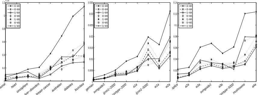
W2: Warm Start By Recycling Old Solution. Besides the cold starts mentioned above, there are

also a couple of simple warm starts possible. To explain these, let us recall that often the hyper-parameterλis chosen by a search over a gridΛ={λ1, . . . ,λm}of candidate values. Let us assume

that these values are ordered in the form λ1>· · ·>λm, and that we train the SVM in the order

λ1, . . . ,λm. Then the resulting n-dimensional vectors C(1), . . . ,C(m)defined by

C_i(j):= (wpos

2λjn if yi=1

wneg

2λjn if yi=−1

have the property C_i(j)<C_i(j+1)for all j=1, . . . ,m−1 and i=1, . . . ,n. For C(1)we can then initialize with one of the above cold starts. Now observe that for j≥2 the approximate solutionα∗obtained by training with Cold:=C(j−1)is feasible for Cnew:=C(j), that is,α∗∈[0,Cnew_{]. Consequently, for} j≥2 we can either initialize with a cold start, or with the warm startα←α∗_{. Obviously, in this}

case we can also recycle∇W(α)and T(α). In addition, the ratio

C_inew C_iold =

λj−1

λj

is independent of i and hence this warm start can be very easily implemented as Procedure 5 shows.

Procedure 5 Initialize byαi←α∗

i and compute∇W(α), S(α), and T(α).

S(α)←T(α∗) +C1new Cold 1

·(S(α∗)−T(α∗))

W4: Warm Start By Partially Expanding And Partially Recycling Old Solution. Apart from

the simple warm start above there is another conceptionally simple warm start for expanding box constraints. Namely, ifα∗denotes an approximate solution to Cold and Cold<Cnewthis warm start initializes byαi←α∗_i ifα∗_i <C_iold and byαi←C_inewifα∗_i =C_iold. The idea behind this warm start is that bounded support vectors, that is, indices in

bSV :={j :α∗_j=Cold_j }

may have the tendency to become larger, when the box constraint is loosened, while unbounded support vectors, that is, vectors in

uSV :={j : 0<α∗_j <Cold_j }

may not have this tendency.

Procedure 6 Initialize bounded SVs byαi←C_inewwhile keeping the rest unchanged and compute ∇W(α), S(α), and T(α).

T(α)←0

E(α)←0

for i=1 to n do

ifαi=C_ioldthen

αi←C_inew

end if end for

if 2·#uSV<#bSV then

for i=1 to n do

∇Wi(α)← C new 1 Cold

1

·∇Wi(α) + 1−C new 1 Cold

1

1−∑j∈uSVαjKi,j

T(α)←T(α)−αi·∇Wi(α)

E(α)←E(α) +C_inew·[∇Wi(α)]2₀

end for else

for i=1 to n do

∇Wi(α)←∇Wi(α) + (Coldi −Cinew)∑j∈bSVKi,j

T(α)←T(α)−αi·∇Wi(α)

E(α)←E(α) +C_inew·[∇Wi(α)]2₀

end for end if

S(α)←T(α) +E(α)

∑j∈bSVα∗jKi,j is simply multiplied by Cinew/Ciold. Recall that the latter ratio is independent of i, and consequently we can update the gradients by either

∇Wi(α)←1−

C₁new C₁old

1−∇Wi(α∗)−

∑

j∈uSV

α∗

jKi,j

−

∑

j∈uSV α∗

jKi,j

for all i=1, . . . ,n, or

∇Wi(α)←∇Wi(α) + (Ciold−Cinew)

∑

j∈bSV

Ki,j, i=1, . . . ,n,

where in the first formula we used

1−∇Wi(α∗)−

∑

j∈uSV

α∗

jKi,j=

∑

j∈bSV

α∗

jKi,j. (10)

require to access some rows of the kernel matrix, and hence there is most likely a more efficient cut-off when only parts of the kernel matrix are stored in memory by caching. Since in general, the costs of computing a row of the kernel matrix depends on data set specific features, such as its dimensionality when using Gaussian kernels, there does not seem to exists a simple rule of thumb in this case, though. Consequently, we decided not to analyze this case carefully. Procedure 6 displays the corresponding pseudocode for this warm start, which we callW4. It is not hard to see, that in the worst case Procedure 6 is

O

(n2_{), while in the best case it is only}

_O

_{(n). Since the average case}

cannot be easily analyzed, we need to experimentally evaluate whether this warm start is efficient or not.

W6: Warm Start By Partially Shrinking And Partially Recycling Old Solution. Let us now

as-sume that we run through the λ-grid in reverse order. Then we have Cold>Cnew, and hence we

Procedure 7 Initialize directions that violate the new box constrained byαi←C_inewwhile keeping

the rest unchanged and compute∇W(α), S(α), and T(α).

for i=1 to n do

ifαi>C_inewthen

αi←C_inew

end if end for

T(α)←0

E(α)←0

if #nuSV <#bSV then

for i=1 to n do

∇Wi(α)←1−C new 1 Cold

1

· 1−∇Wi(α)−∑j∈nuSVα∗jKi,j−∑j∈nbSVα∗jKi,j

∇Wi(α)←∇Wi(α)−∑j∈nuSVα∗jKi,j−∑j∈nbSVCnewj Ki,j

T(α)←T(α)−αi·∇Wi(α)

E(α)←E(α) +C_inew·[∇Wi(α)]2₀

end for else

for i=1 to n do

∇Wi(α)←∇Wi(α) +∑j∈bSV(Coldj −Cnewj )Ki,j ∇Wi(α)←∇Wi(α) +∑j∈nbSV(α∗j−Cnewj )Ki,j

T(α)←T(α)−αi·∇Wi(α)

E(α)←E(α) +C_inew·[∇Wi(α)]20

end for end if

S(α)←T(α) +E(α)

cannot immediately recycle the old approximate solutionα∗. Nonetheless, there is a certain ana-logue to Procedure 6 possible. Indeed, we can initialize byαi←α∗

split the set uSV into

nuSV := {j : 0<α∗_j≤Cnew_j }, nbSV := {j : Cnew_j <α∗_j<Cold_j },

where we note that we use a slight abuse of the letters u and b in this notation. Now note that the initialization above multiplies all α∗_j ∈bSV by the factor C₁new/Cold

1 , while it keeps allα∗j ∈nuSV unchanged. Obviously, both update rules make it possible to recycle parts of the gradient. Un-fortunately, however, forα∗_j ∈nbSV, the situation is more complicated and no simple recycling is

possible. Thus, Procedure 7, which displays the corresponding pseudocode, is a little more com-plicated than Procedure 6. Nonetheless, all remarks concerning the computational requirements of Procedure 6 also apply to Procedure 7, and the same holds true for the rule that decides which part of the gradient is recycled. In the following, we call this approach displayed in Procedure 7,W6.

W3 & W5: Warm Start By Scaling Old Solution. Finally, there is an easy warm start option that

works regardless of the direction we run through the λ-grid. Indeed, we can always initialize by αi ←α∗_i ·Cnew

1 /Cold1 . The Procedure 8 shows the corresponding

O

(n) pseudocode. Depending on

whether C₁old<C₁newor C₁old>C₁newwe call this approachW3orW5, respectively.

Procedure 8 Initialize byαi←α∗_i ·Cnew

1 /C1oldand compute∇W(α), S(α), and T(α). T(α)←0

E(α)←0

for i=1 to n do

αi←Cnew1 Cold 1

·α∗

i ∇Wi(α)←1−

Cnew 1 Cold

1

· 1−∇Wi(α)

T(α)←T(α)−αi·∇Wi(α)

E(α)←E(α) +C_inew·[∇Wi(α)]20

end for

S(α)←T(α) +E(α)

3. Working Sets of Size Two

So far, our algorithm performs an update in one coordinate per iteration. Let us now consider an algorithm which performs an update in two coordinates per iteration. To this end, let us first present the following, simple lemma that computes the gain of a 2-dimensional update.

Lemma 2 Forδi,δj∈Rand i,j=1, . . . ,n we have

W(α+δiei+δjej)−W(α) =δi·(∇Wi(α)−δi/2) +δj·(∇Wj(α)−δj/2)−δiδjKi,j.

Proof Applying Lemma 1 twice and using the formula∇Wj(α+δiei) =∇Wj(α)−δiKi,j we find

3.1 Solving the Two-Dimensional Problem Exactly

In order to describe an algorithm that updates two variables at each iteration we first have to in-vestigate how the two-variable update looks like in detail. To this end, we fix two coordinates

i,j∈ {1, . . . ,n}with i6= j and consider the function

(αi˜ ,α˜j)7→Wi,j(αi˜ ,α˜j):=W(α\i,j+αi˜ ei+α˜jej),

whereα\i,j:=α−αiei−αjejis a fixed vector whose i-th and j-th coordinates equal zero. A simple calculation then shows

Wi,j(αi˜ ,α˜j) = he,α\i,ji+αi˜ +α˜j− 1 2hα

\i,j_,Kα\i,j_{i −αi˜ he}

i,Kα\i,ji −α˜jhej,Kα\i,ji

−1

2 α˜

2

i +2 ˜αiα˜jKi,j+α˜2j

,

where we used Ki,i=Kj,j=1. Consequently, the partial derivatives are given by

∂Wi,j(αi˜ ,α˜j)

∂αi˜ = 1− hei,Kα

\i,j_{i −αi˜ −α˜} jKi,j,

∂Wi,j(αi˜ ,α˜j) ∂α˜j

= 1− hej,Kα\i,ji −α˜j−αi˜ Ki,j.

In order to derive the maximum of Wi,jon[0,Ci]×[0,Cj]from these derivatives, we need to consider three different cases.

The Case Ki,j=1. By setting the above derivatives to zero, we obtain the following system of linear equations

α∗

i +α∗j = 1− hei,Kα\i,ji, α∗

i +α∗j = 1− hej,Kα\i,ji

that have to be satisfied for all global maxima(α∗_i,α∗_j)∈R2of Wi,j. Now recall that we assumed that

the kernel k is strictly positive definite, and therefore we see that Ki,j=1 implies xi=xj, and hence

yi=yj. From this we conclude Ki,ℓ=Kj,ℓfor allℓ=1, . . . ,n, and thus we obtain 1− hei,Kα\i,ji= 1− hej,Kα\i,ji. Consequently, Wi,jattains its global maximum at every point of the affine subspace

(α∗_i,α∗_j):α∗_i +α∗_j=1− hei,Kα\i,ji , (11)

which is a translated version of the anti-diagonal subspace{(α,−α):α∈R}.

Now recall that yi=yj implies Ci=Cj, and hence we are actually interested in finding a pair

(αi˜ ,α˜j)that maximizes Wi,j on the square[0,Ci]2. If 1− hei,Kα\i,ji ∈[0,2Ci], it is easy to see that the subspace (11) intersects the square, and hence Wi,jattains the desired maximum at every element in this intersection. In particular,(α∗

i,α∗i), where

α∗

i :=

1− hei,Kα\i,ji 2

of the set of edges{Ci} ×[0,Ci]∪[0,Ci]× {Ci}. Let us fix a pair(αi˜ ,α˜j)∈ {Ci} ×[0,Ci]. Then we have

∂Wi,j(αi˜ ,α˜j) ∂α˜j

=1− hej,Kα\i,ji −α˜j−αi˜ Ki,j=1− hej,Kα\i,ji −α˜j−Ci>0,

and hence Wi,j attains its maximum over{Ci} ×[0,Ci]at the corner(Ci,Ci). Interchanging the roles of i and j we can thus conclude that Wi,j attains its maximum over[0,Ci]2at(Ci,Ci). Since we can analogously show that, for 1− hei,Kα\i,ji<0, the function Wi,j attains its maximum over[0,Ci]2at

(0,0), we finally find the update rule

αnew

i :=αnewj :=

1− hei,Kα\i,ji 2

Ci

0 =

∇

Wi(α) +αi+αj 2

Ci

0 .

The Case Ki,j=−1. In this case, we have xi=xj, and hence yi=−yj. From this we conclude

Ki,ℓ=−Kj,ℓfor allℓ=1, . . . ,n, and thus we obtainhei,Kα\i,ji=−hej,Kα\i,ji. Consequently, the derivatives above reduce to

∂Wi,j(αi˜ ,α˜j)

∂αi˜ = 1− hei,Kα

\i,j_{i −αi˜ +α˜} j,

∂Wi,j(αi˜ ,α˜j) ∂α˜j

= 1+hei,Kα\i,ji −α˜j+αi˜ ,

and from this it is easy to conclude that Wi,j does not have a global maximum. However, a closer inspection of Wi,jyields the formula

Wi,j(αi˜ ,α˜j) =he,α\i,ji+αi˜ +α˜j− 1 2hα

\i,j_,Kα\i,j_{i −(αi˜ −α˜}

j)hei,Kα\i,ji − 1

2 αi˜ −α˜j

2 ,

and hence we see that, for fixedβ∈R, we have

Wi,j(αi˜ ,αi˜ +β) =he,α\i,ji+2 ˜αi+β− 1 2hα

\i,j_,Kα\i,j_i+βhe

i,Kα\i,ji − 1 2β

2_.

In other words, Wi,jis a affine linear function with positive slope on the affine subspaces

{(αi˜ ,αi˜ +β): ˜αi∈R}, β∈R,

and therefore Wi,j attains its maximum over[0,Ci]×[0,Cj]at a point from the set of edges{Ci} ×

[0,Cj]∪[0,Ci]× {Cj}. Let us first consider a pair(αi˜ ,α˜j)∈ {Ci} ×[0,Cj]. Then we have

∂Wi,j(αi˜ ,α˜j) ∂α˜j

=1− hej,Kα\i,ji −α˜j+Ci,

and hence Wi,j attains its maximum over{Ci} ×[0,Cj]at(Ci,α∗j), where

α∗

j = [1− hej,Kα\i,ji+Ci] Cj

0 = [∇Wj(α) +αj−αi+Ci]

Cj 0 .

Moreover, for δi :=Ci−αi and δj :=α∗j−αj we obtain the gain of this update by Lemma 2. Analogously, we can show that Wi,jattains its maximum over[0,Ci]× {Cj}at(α∗i,Cj), where

α∗

Again, the gain of the corresponding update can be computed by Lemma 2, and by comparing both gains we can then decide which two-dimensional update yields the larger gain. The corresponding update is chosen in the algorithm.

The Case Ki,j6=±1. To solve the two dimensional problem in this case we fix anα∈Rnand write

γi := 1− hei,Kα\i,ji=1−

∑

ℓ6=i,j

αℓKi,ℓ=∇Wi(α) +αi+αjKi,j,

γj := 1− hej,Kα\i,ji=1−

∑

ℓ6=i,j

αℓKj,ℓ=∇Wj(α) +αj+αiKi,j.

Using the derivatives of Wi,j it is then easy to see that Wi,j attains its global maximum at each point(α∗

i,α∗j)that satisfiesγi=α∗i +α∗jKi,j andγj =α∗j+α∗iKi,j. Furthermore, simple algebraic transformations show

α∗

i =

γi−γjKi,j

1−K_i2_,j and α ∗

j=

γj−γiKi,j 1−K_i2_,j ,

and by re-substituting the definition ofγiandγjwe hence obtain

α∗

i = αi+

∇Wi(α)−∇Wj(α)Ki,j

1−K2

i,j ,

α∗

j = αj+∇

Wj(α)−∇Wi(α)Ki,j 1−K2

i,j

(12)

for the uniquely determined point at which Wi,j attains its global maximum. Now if (α∗i,α∗j)∈

[0,Ci]×[0,Cj]we can simply update by(αnewi ,αnewj ):= (α∗i,α∗j). However, if(α∗i,α∗j)6∈[0,Ci]×

[0,Cj]we have to make further calculations. For example, forα∗i >Ciandα∗j ∈[0,Cj], the function

Wi,j attains its maximum over[0,Ci]×[0,Cj]at a point of the line{Ci} ×[0,Cj]by the concavity of

Wi,j. Consequently, in this case the update is

(αnew_i ,αnew_j ):= Ci,[∇Wj(α) + (αi−Ci)Ki,j+αj] Cj 0

,

that is, we first update the i-th coordinate, which leads to the temporary gradient

∇Wj(α) + (αi−Ci)Ki,j,

and then perform a one-dimensional optimization over the j-th coordinate. The remaining three cases where exactly one direction of(α∗_i,α∗_j)violates the box constraint can be handled analogously. Finally, let us consider the cases, where both coordinates violate the constraint, for example,α∗_i >Ci andα∗_j >Cj. In this case, the concavity of Wi,j shows that Wi,j attains its maximum over[0,Ci]×

Algorithm 22D-SVMsolver initialize α,∇W(α),T(α),S(α)

while S(α)>₂ε_λdo

select directions i∗and j∗

updateαin the directions i∗and j∗

update∇W(α)in the directions i∗and j∗and calculate T(α)and E(α) S(α)←T(α) +E(α)

end while

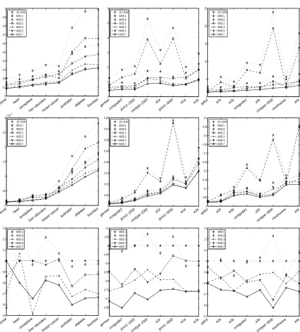
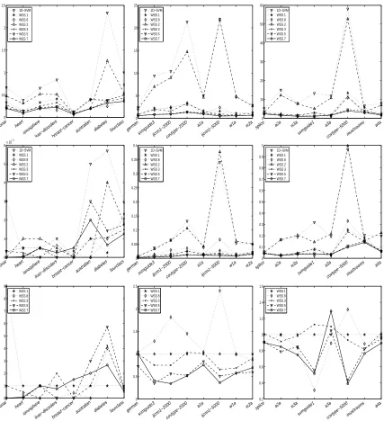
3.2 Selecting a Working Set of Size Two

The 2D-SVM-solver displayed in Algorithm 2 is conceptionally very similar to the1D-SVM-solver presented in Algorithm 1. However, so far we have not addressed how to choose the directions i∗ and j∗ in which the2D-SVM-solver performs an update. Obviously, several possibilities exists for this task, and we discuss a few of them in the following.

WSS 0: Choose The Pair Of Directions With Maximal Gain. Given a pair of directions(i,j),

Lemma 2 can be used to compute the gain of W resulting from the exact two dimensional optimiza-tion described in Secoptimiza-tion 3.1. Now one could consider all pairs of direcoptimiza-tions and choose the one with the largest gain. Of course, in practice this approach is prohibitive, since the search is an

O

(n2)

operation, which has to be performed in each iteration. Nonetheless, in some sense this approach may be viewed as an “optimal” two dimensional strategy, and all subset selection strategies devel-oped below can be interpreted as low cost approximations to this approach. Consequently, we tested it to get a baseline number of iterations, to which all other subset selection strategies are compared to.

WSS 1: 1D-direction With Maximal Gain And Previously Found 1D-direction. A careful

anal-ysis of the behavior of the1D-SVM-solver shows that it often comes into a regime in which it picks alternating indices i∗ and j∗ for a while. In other words, it tries to approximately solve the 2D-problem in the directions i∗and j∗. In order to avoid this cost-intensive alternating we can look for the best 1D-direction i∗and then perform a 2D-update over i∗ and the 1D-direction i∗_old chosen in the previous iteration. Conceptionally, this approach is very close to the maximum-gain procedure mentioned in Glasmachers and Igel (2006) for SVMs with offset. The advantage of this approach is that it preserves the low-cost search from the1D-SVM-solver. On the downside, however, it may not reduce the number of iterations very effectively.

WSS 2: Two 1D-directions With Maximal Gain From Separate Subsets. Another simple way

to preserve the low cost search from the1D-SVM-solver is to split the index set{1, . . . ,n}into two parts{1, . . . ,n/2} and{n/2+1, . . . ,n} and search for the 1D-directions with maximal gain over these two parts separately. In other words, we can choose the directions i∗and j∗by

i∗ ∈ arg max

i≤n/2W(α+δiei)−W(α), j∗ ∈ arg max

i>n/2W(α+δiei)−W(α),

WSS 4: 1D-direction With Maximal Gain And A Direction Of A Nearby Sample. Yet another

approach to preserve the low cost search from the1D-SVM-solver is to first look for the 1D-direction

i∗with maximal gain, and then, in a second step, to pick a direction j∗ such that xj∗ is close to x_i∗ with respect to the metric

dk(x,x′):=

p

2−2k(x,x′_{), x,x}′_∈X,

induced by the kernel. Note that x is close to x′ in this metric, if and only if k(x,x′)is close to 1. Consequently, the gradients of the samples close to xi∗ are the ones that are most affected by an update in direction i∗. Therefore, if these gradients are close to zero before the update, they will most likely be no longer close to zero after the update, and hence the corresponding directions will have a good chance of being chosen in a subsequent iteration. In our experiments, we considered the

k-nearest neighbors of x∗_i, where k=10, and picked the neighbor xj∗for which the 2D-update in the directions(i∗,j∗)yielded the largest gain. Note that, as soon as the direction i∗is found, it is clear that one subsequently needs to access the i∗-th kernel row for updating the gradient. Therefore, this working set selection strategy does not require further kernel computations. Moreover, computing the 2D-gain over k candidates is also relatively inexpensive, if k remains small. Nonetheless, initial experiments suggested that searching over the k-nearest neighbors only makes sense when the solver mainly updates inner support vectors, that is, directions i with 0<αi <Ci. Consequently, we implemented a Boolean flag that was recomputed every 10 iterations. In this re-computation, the flag was set to true, if and only if in at least 5 of the previous 10 iterations the picked directions

i∗and j∗both were inner support vectors. We then considered the k-nearest neighbors only if this Boolean flag was set, while in the other case we applied the working set selection strategyWSS 1.

WSS x:Combinations Of 1D-direction-based Approaches. It is easy to see that one can combine

the previous three methods that are based on finding the 1D-direction with maximal gain. For example, in each iteration one can combineWSS 1andWSS 2by computing the 2D-gain of both methods and pick the one with the larger gain. Obviously, this still preserves the low cost search from the1D-SVM-solver and only adds little cost for computing the 2D-gain for the two candidate pairs. Similarly, all three methods can be combined. Combinations of these methods are called

WSS x, wherexis the sum of the combined methods. For example, by combiningWSS 1,WSS 2,

andWSS 4we obtainWSS 7, and by combiningWSS 1,WSS 2,WSS 4withWSS 512below, we

obtainWSS 519. In the following, we keep this binary numbering system which makes it possible to easily describe arbitrary combinations of basic working set selection strategies.

WSS 8: 1D-direction With Maximal Gain And One-step-ahead 1D-direction. Another way to

extend the1D-SVMsubset selection strategy to two directions is to first look for the 1D-direction i∗ with maximal gain, and then to look for the 1D-direction j∗with maximal gain that would be found after having updated in direction i∗. Obviously, this strategy, which we callWSS 8, is closely related

toWSS 1in that the update and search routines are partially permuted. However, it has a higher

cost for the search part per iteration, while intuitively it should reduce the number of iterations.

WSS 16: Maximal Violating Pair. A completely different subset selection strategy is based on

updated in every iteration. This may add some cost per iteration compared to the previous working set selection strategies, while it is unclear how the number of iterations behave compared to these strategies.

WSS 32: 1D-direction With Maximal Gain And Corresponding “Optimal” 2D-direction. None

of the methods introduced so far try to seriously approximate the 2D-subset selection strategyWSS 0, which intuitively picks the best possible pair of indices. The first method that seriously strives for such an approximation is WSS 32, which first picks the 1D-direction i∗ with maximal gain, and then searches for the j∗∈ {1, . . . ,n} such that(i∗,j∗)maximizes the corresponding 2D-gain. Obviously, the cost for this search method is significantly higher than those ofWSS 1toWSS 7, but it is still

O

(n). On the other hand, the better choice of(i∗,j∗)may substantially reduce the number of iterations of the2D-SVM-solver, and hence it is not a-priori clear howWSS 32performs compared to the earlier methods. Finally, note thatWSS 32is related to the second order working set selection strategy of Fan et al. (2005), which was proposed for SVMs with offset.

WSS 64: 1D-direction With Maximal Gain And Random “Optimal” 2D-direction. Instead of

considering all pairs(i∗,j), j=1, . . . ,n, asWSS 32does, it may suffice to reduce the search over the pairs(i∗,j), j∈J, where J⊂ {1, . . . ,n}is a random subset. In our experiments we considered the case #J=n/5.

WSS 128: 1D-direction With Maximal Gain And Approximately “Optimal” 2D-direction. One

of the disadvantages ofWSS 32is that computing the 2D-gain is quite expensive due to the relatively large number of branches and floating point operations. One way to address this issue is to compute the 2D-gain inWSS 32only approximately.WSS 128uses the following approximation: for indices

i and j with Ki,j=±1 it computes the exact gain, while for the other pairs it first computesα∗i and α∗

j by (12), and then applies the simple clipping operation

αnew

i := [α∗i]

Ci 0 ,

αnew

j := [α∗j]

Cj 0 .

For these newα’s,WSS 128finally computes the gain by Lemma 2. Clearly, this gain is in general less than the exact gain, but it still may be a good approximation. In particular, if both α∗_i and α∗

j satisfy the box constraints, then the approximation is actually exact. On the other hand, the approximation is clearly less expensive, but we expect more iterations compared toWSS 32.

WSS 256: Random 2D-directions With Maximal Gain. Another way to approximateWSS 0is

to consider k random pairs(i,j), and pick the pair(i∗,j)that yields the largest exact 2D-gain among them. InWSS 256we followed this idea for k :=n.

WSS 512: 1D-direction With Maximal Gain And 2D-direction Over Inner SVs. Although the

approximate computation of the 2D-gain inWSS 128is cheaper than the exact computation inWSS 32, it may still be too expensive. One way to further decrease these costs is based on the observation that the 2D-gain is given by

1 2·

|∇Wi(α)|2+|∇Wj(α)|2−2∇Wi(α)∇Wj(α)Ki,j 1−K_i2_,j

set,WSS 512searches for the direction

j∗∈ {j : 0<αj<Cjand Ki∗_,j6=±1}

that optimizes the above formula of the 2D-gain for fixed i :=i∗. Since in some iterationsWSS 512reduces to the1D-SVM-solver we further considered some combinations withWSS 3, andWSS 7in our experiments. Following the naming convention of combinations mentioned earlier, these strategies are calledWSS 515andWSS 519.

WSS 1024: 1D-direction With Maximal Gain And Random 2D-direction Over Inner SVs. The

next subset selection strategy, WSS 1024, is quite similar to WSS 512, except that it does not consider all inner support vectors in the search for j∗, but only k random inner support vectors. In our experiments we used the k that equaled 20% of the current number of inner support vectors. In addition, we initiated the search wheneverαi∗ was an inner support vector, that is, the search was initiated independently of the Boolean flag ofWSS 4. Again, in some iterationsWSS 1024reduces to the1D-SVM-solver, and hence we further considered some combinations with WSS 1, WSS 2,

andWSS 4, where again the naming convention above was used.

WSS 2048: Add Random 2D-directions Over Inner SVs. The final subset selection strategy,

WSS 2048, is actually not a subset selection strategy of its own, but only a strategy that works in

combination with others. Once one of the previous subset selection strategies has picked a pair

(i∗,j∗)andαi∗ has turned out to be an inner support vector,WSS 2048considers k random pairs of inner support vectors, and picks the pair(i∗∗,j∗∗)that has largest approximate gain, where the ap-proximation was computed as inWSS 512. Then the exact gain of(i∗,j∗)and(i∗∗,j∗∗)is computed and the pair with the larger exact gain was chosen. We considered this method in combination with

WSS 1,WSS 2, andWSS 4, where again the naming convention above was used.

4. Convergence Analysis

In this section we establish an upper bound on the number of iterations for both the1D-SVMand the

2D-SVM. Our approach is heavily based on earlier ideas2developed for the analysis of rate-certifying decomposition algorithms, see, for example, Hush and Scovel (2003), List and Simon (2005), Hush et al. (2006) and List and Simon (2007), but it may be possible to partially use results on block coordinate descent algorithms such as the one by Luo and Tseng (1992) for the analysis, instead.3

Let us begin by recalling from the first papers mentioned that the σ-functional for a vector α∈[0,C] = [0,C1]× · · · ×[0,Cn]and an index set I⊂ {1, . . . ,n}is defined by

σ(α|I):= sup

˜

α∈[0,C]

˜

αi=αi∀i6∈I

∇

W(α),α˜−α .

2. Despite this, we decided to include the analysis, since: a) it still requires a little work and thus we felt that it was a bit unfair to the reader to simply say that the analysis is straightforward; b) we thought that it was nice to see how the relatively complicated techniques for the offset case significantly simplify; c) our goal was to provide a full and self-contained work for the proposed algorithm.

Since our algorithms are based on gain optimization rather than rate certification, we further need theγ-functional

γ(α|I):= sup

˜

α∈[0,C]

˜

αi=αi∀i6∈I

W(α˜)−W(α),

which expresses the gain in the dual objective function resulting from an optimization over the directions contained in I. To simplify notations, we writeσ(α|i):=σ(α|{i})andγ(α|i):=γ(α|{i}). Note that we have

σ(α|i) = sup

˜

αi∈[0,Ci]

(αi˜ −αi)∇Wi(α),

whileγ(α|i)expresses the gain

W α+ (αnew_i −αi)ei

−W(α)

of the 1D-update in direction i, where αnew_i is defined by (4). In addition, γ(α|{i,j}) is the gain obtained by the update discussed in Section 3.1. Moreover, for I={1, . . . ,n} we writeσ(α):=

σ(α|I)andγ(α):=γ(α|I), respectively. Note that bothσandγare monotonic in I, that is, for I⊂J

we haveσ(α|I)≤σ(α|J)andγ(α|I)≤γ(α|J). Finally, we need the obvious relation

γ(α) =W(α∗)−W(α),

where we recall from Section 2 thatα∗∈[0,C]denotes a solution of the dual problem (3). In other words,γ(α)expresses the dual sub-optimality ofα.

Let us now begin our analysis by presenting two lemmata that establish relationships between these quantities.

Lemma 3 For allα∈[0,C]we have

n

∑

i=1

σ(α|i) =σ(α) =gap(α),

where gap(α) denotes the duality gap defined in (7). In particular, there exists an index i⋆ ∈ {1, . . . ,n}such that

σ(α|i⋆)≥n−1σ(α).

This lemma can be easily derived from results in List et al. (2007) and List and Simon (2007). However, in the case of SVMs without offset, its proof is very elementary and hence we present it here for the sake of completeness.

Proof For i∈ {1, . . . ,n}it is easy to see that the supremum used to defineσ(α|i)is attained at

¯ αi:=

(

Ci if∇Wi(α)≥0 0 if∇Wi(α)<0.

(13)

Moreover, the vector ¯α:= (α¯₁, . . . ,αn¯ )∈[0,C]realizes the supremum definingσ(α), and hence we obtain

n

∑

i=1

σ(α|i) =

n

∑

i=1 ∇

W(α),(αi¯ −αi)ei

Furthermore, we have

σ(α) =h∇W(α),α¯−αi = hα,Kαi − he,αi+

n

∑

i=1

¯

αi·∇Wi(α)

= hα,Kαi − he,αi+

n

∑

i=1

Ci[∇Wi(α)]∞0,

and therefore we have shownσ(α) =gap(α). The last assertion is a trivial consequence of the first assertion.

The second lemma relatesσ(α|I)to the gainγ(α|I). For its formulation we need the quantity

Bmax:=maxi=1,...,nCi.

Lemma 4 For allα∈[0,C]and I⊂ {1, . . . ,n}we have

σ(α|I) ≥ γ(α|I) ≥ σ(α|I)

2 min

1, σ(α|I) |I|2_B2

max

,

where|I|denotes the cardinality of I.

In a slightly different form, this lemma has been established in, for example, Hush et al. (2006), and it was somewhat implicitly used in List and Simon (2007). Again, we present its proof for the sake of completeness.

Proof Let ¯αibe defined by (13) and d :=∑i_∈I(αi¯ −αi)ei. Forλ∈[0,1], we then haveα+λd∈[0,C],

and a calculation analogous to the one in the proof of Lemma 1 yields

γ(α|I)≥W(α+λd)−W(α) =λ∇

W(α),d −λ

2

2hd,Kdi ≥λσ(α|I)−

λ2_|I|2_B2 max

2 .

Now the right hand side is maximized at

λ∗_:= (

1 ifσ(α|I)>|I|2_B2 max |I|−2_B−2

maxσ(α|I) ifσ(α|I)≤ |I|2B2max.

In the caseσ(α|I)>|I|2_B2

maxwe hence find

γ(α|I)≥σ(α|I)−|I| 2_B2

max

2 > σ(α|I)

2 ,

while in the other caseσ(α|I)≤ |I|2_B2

maxwe obtain

γ(α|I)≥ σ 2₍α_|I)

2|I|2_B2 max

.

Combining all estimates we then obtain the inequality on the right hand side.

To show the inequality on the left hand side we fix an ˜α∈[0,C]such that ˜αi=αi for all i6∈I.

Then we have

W(α˜)−W(α) =h∇W(α),α˜ −α)−1

and by maximizing the left hand side of this inequality over ˜αwe findγ(α|I)≤σ(α|I).

With these preparations we can now present a preliminary result on iterative algorithms that have a certain control of their gain.

Proposition 5 Letα(0),α(1)_{,· · · ∈[0,C]be a sequence of feasible vectors that satisfies}

W(α(ℓ+1))−W(α(ℓ))≥γ(α(ℓ)|i⋆_ℓ), ℓ≥0, (14)

where for each ℓ the index i⋆_ℓ ∈ {1, . . . ,n} is the one described in Lemma 3, that is, it satisfies

σ(α(ℓ)|i⋆_ℓ)≥n−1σ(α(ℓ)). Then for allℓ≥1 we have

γ(α(ℓ+1))≤γ(α(ℓ))

1− 1

2nmin

1,γ(α

(ℓ)₎

nB2 max

.

Moreover, for allε>0 and allℓ≥ℓ_εwe haveγ(α(ℓ))≤ε, where

ℓ_ε:=

2n2B2_max

ε

+max

0,

2n lnW(α

∗_)−W(α(0)₎

ε

.

Proof By Lemmas 4 and 3 we find

γ(α(ℓ))−γ(α(ℓ+1)) =W(α(ℓ+1))−W(α(ℓ)) ≥ γ(α(ℓ)|i⋆_ℓ) ≥ σ(α

(ℓ)_|i⋆ ℓ)

2 min

1,σ(α

(ℓ)_|i⋆ ℓ)

B2 max

≥ σ(α

(ℓ)₎

2n min

1,σ(α

(ℓ)₎

nB2 max

≥ γ(α

(ℓ)₎

2n min

1,γ(α

(ℓ)₎

nB2 max

.

From this we easily obtain the first assertion.

The second assertion has already been shown in the second part of the proof of the first assertion of (List and Simon, 2007, Theorem 4), which can be found on the pages 312 and 313 of List and Simon (2007).

Note that 1/n-rate certifying algorithms considered in List and Simon (2007) clearly satisfy

assumption (14). Moreover, Proposition 5 can also be applied to the1D-SVMand2D-SVM:

Theorem 6 Consider the1D-SVMdescribed in Algorithm 1 or a2D-SVMin the sense of Algorithm

2 that uses a working set selection strategy whose gain at each iteration is not less than that of the 1D-SVM. Furthermore, assume that max{w_neg,w_pos} ≤1. Then for allε>0, n≥1, and allλ>0

these algorithms terminate after at most

2 λεmin{1,2λε}

+max

0,

2n ln4λ(W(α

∗_)−W(α(0)₎₎

εmin{1,2λε}

iterations. In particular, in the most likely scenario 2λε≤1 these algorithms do not need more

iterations than

1 λ2ε2

+max

0,

2n ln2(W(α

∗_)−W(α(0)₎₎

ε2

.

Proof The1D-SVMchooses at each iterationℓa direction i∗_ℓ that maximizes the 1D-gainγ(α(ℓ)|i).

Consequently, we have

W(α(ℓ+1))−W(α(ℓ)) =γ(α(ℓ)|i∗_ℓ)≥γ(α(ℓ)|i⋆_ℓ),

where i⋆_ℓ is the direction described in Lemma 3. In other words, (14) is satisfied for this algorithm, and from this it is not hard to see that the considered2D-SVM’s also satisfy assumption (14). Let us now define

h(σ):= σ

2min

1, σ n2_B2

max

, σ>0.

Forε:=h(₂ε_λ)Proposition 5 together with Lemma 4 then shows that

h ε

2λ

=ε≥γ(α(ℓ))≥h σ(α(ℓ))

for allℓ≥ℓ_ε and hence we obtain S(α(ℓ))≤gap(α(ℓ)) =σ(α(ℓ))≤ ₂ε_λ by the monotonicity of the function h. Using Bmax≤_2λn1 we then obtain the assertion by simple algebraic transformations.

Note that the working set selection strategiesWSS 1,WSS 2,WSS 4,WSS 8,WSS 32,WSS 64,

WSS 128,WSS 512, andWSS 1024, satisfy the assumptions of Theorem 6. Moreover, the same is true for all combinations of working set selection strategies that include at least one of the strategies listed. Finally, note that the upper bound established in Proposition 5 coincide (modulo constants that come from different working set sizes) with the bounds for rate certifying algorithms presented in List and Simon (2005), Hush et al. (2006) and List and Simon (2007). Moreover, the step from dualε-optimality to primalε-optimality considered in the proof of Theorem 6 coincides with the analysis (List et al., 2007) for SVMs with offset. Consequently, the bound presented in Theorem 6 equals the best known guarantees for solvers for SVMs with offset.

5. Experiments

The described 1D-SVM-solver and 2D-SVM-solver enjoy nice theoretical properties with respect to both generalization performance and required training time. However, it is unclear how tight these bounds are, so it remains unclear whether the proposed SVMs also perform well in practice. Therefore, we performed several experiments that address the following questions:

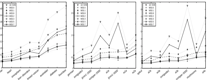
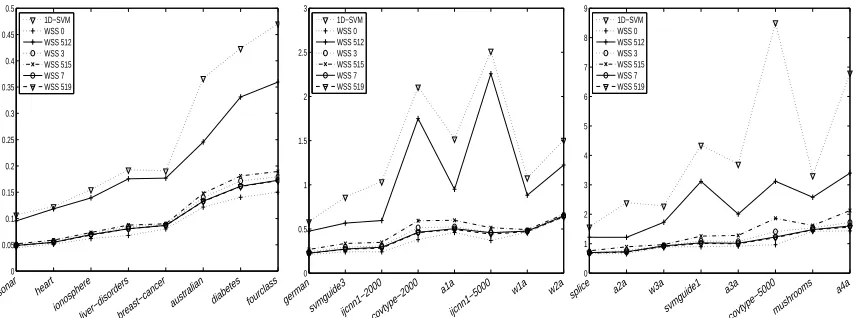
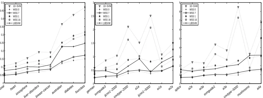
1. Which subset selection strategies lead to the smallest number of iterations or the shortest run time? How many more iterations thanWSS 0do these strategies perform?

2. How many less iterations needs the stopping criterion (9) compared to standard duality gap (7) and is there also an advantage in terms of run time?

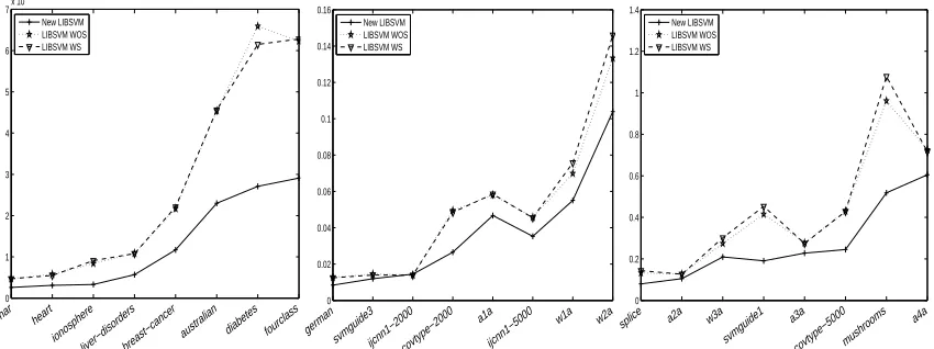
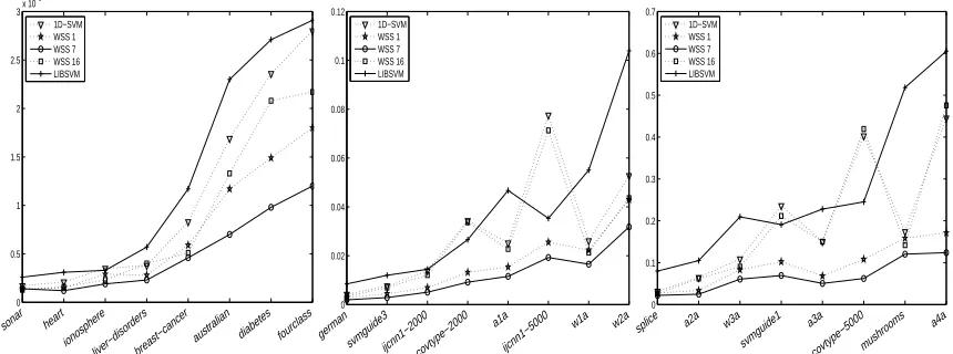
4. How well does the 2D-SVM-solver work compared to standard software packages such as

LIBSVMby Chang and Lin (2009)?

5. What is the advantage of warm start initializations when the parameter search is performed over a grid?

To answer these questions we implemented the1D-SVM- and the2D-SVM-solver in C++, and down-loadedLIBSVMversion 2.82 by Chang and Lin (2009). The algorithms were compiled by LINUX’s gccversion 4.3 with various software and hardware optimizations enabled. All experiments were conducted on a computer with INTEL XEON X5355 (2.66 GHz) quad core processor and 8GB RAM under a 64bit version of RedHat Linux Enterprise 4. During all experiments that incorpo-rated measurements of run time, one core was used solely for the experiments, and the number of other processes running on the system was minimized. The run time itself was measured by the C functionclock()from the librarytime.h. The resulting resolution was 0.01 seconds.

In some preliminary experiments we made a couple of observations that changed the described implementation strategy slightly: First, it turned out that the auto-vectorization of gcconly gave mediocre and sometimes even contradicting results, even if the implementation guidelines ofgcc 4.3’s auto-vectorization were strictly followed. Therefore, we decided to manually code SSE2 -vectorized versions of the most important routines, namely: computing kernel values, searching for the optimal 1D-direction, updating the gradient, and computing the weighted sum E(α)of clipped slack variables. To this end, we used the libraryemmintrin.htogether with properly aligned arrays of doubles.4 Some of our preliminary experiments not reported here indicated that this specialized hardware instruction set yields a run time improvement by a factor between 1.3 and 1.8 depending on the working set selection strategy and the data set. Second, the initial experiments suggested substantial numerical instabilities on a few data sets when using single floats, so we decided to use double precision throughout the experiments. Third, we were rather disappointed by the run time behavior ofLIBSVM, even when we enabled its shrinking heuristic.5After some investigations we found that the main reason for the disappointing run time performance was the fact that LIB-SVMcopies kernel rows into the kernel cache, if one uses pre-computed kernel matrices, which, as discussed below, we did throughout the experiments. This copying mechanism results in a small number of iterations per second when theLIBSVM-solver is started on a new parameter point, while with the kernel cache being filled up during the optimization, the solver starts performing more it-erations per second. To ensure a fair comparison, we thus decided to implement our own version of

LIBSVM’s solver (without shrinking strategy). As a side effect, this new implementation also

ben-efited from theSSE2instructions for upgrading the gradient. Unlike the subset selection strategy of the 1D-SVM-solver, however, LIBSVM’s subset selection strategy, though implementable, does

4. At first glance, this manual approach may seem to be too specialized, since it should clearly be not the goal of this paper to fine-tune an algorithm to a very specific hardware environment. On the other hand, a good compiler should

make optimizations with respect to these nowadays standard instructions, which have been first introduced byIntelin

2001 and have been adopted byAMDin 2003, automatically. Unfortunately, it turned out thatgcc4.3 did not do this

optimization reliably. Namely, depending on some minor and apparently independent changes in other parts of the code, the most crucial loops where sometimes optimized and sometimes not. This behavior rendered a reasonable comparison of different algorithms impossible. Therefore, our manual approach can also be viewed as a compilation with a more ideal compiler, which in the future is hopefully available.