Adaptive Subgradient Methods for Online Learning and Stochastic Optimization

Adaptive Subgradient Methods for

Online Learning and Stochastic Optimization

John Duchi [email protected]

Computer Science Division University of California, Berkeley Berkeley, CA 94720 USA

Elad Hazan [email protected]

Technion - Israel Institute of Technology Technion City

Haifa, 32000, Israel

Yoram Singer [email protected]

Google

1600 Amphitheatre Parkway Mountain View, CA 94043 USA

Editor: Tong Zhang

Abstract

We present a new family of subgradient methods that dynamically incorporate knowledge of the geometry of the data observed in earlier iterations to perform more informative gradient-based learning. Metaphorically, the adaptation allows us to find needles in haystacks in the form of very predictive but rarely seen features. Our paradigm stems from recent advances in stochastic op-timization and online learning which employ proximal functions to control the gradient steps of the algorithm. We describe and analyze an apparatus for adaptively modifying the proximal func-tion, which significantly simplifies setting a learning rate and results in regret guarantees that are provably as good as the best proximal function that can be chosen in hindsight. We give several efficient algorithms for empirical risk minimization problems with common and important regu-larization functions and domain constraints. We experimentally study our theoretical analysis and show that adaptive subgradient methods outperform state-of-the-art, yet non-adaptive, subgradient algorithms.

Keywords: subgradient methods, adaptivity, online learning, stochastic convex optimization

1. Introduction

In many applications of online and stochastic learning, the input instances are of very high di-mension, yet within any particular instance only a few features are non-zero. It is often the case, however, that infrequently occurring features are highly informative and discriminative. The infor-mativeness of rare features has led practitioners to craft domain-specific feature weightings, such as TF-IDF (Salton and Buckley, 1988), which pre-emphasize infrequently occurring features. We use this old idea as a motivation for applying modern learning-theoretic techniques to the problem of online and stochastic learning, focusing concretely on (sub)gradient methods.

Standard stochastic subgradient methods largely follow a predetermined procedural scheme that is oblivious to the characteristics of the data being observed. In contrast, our algorithms dynamically incorporate knowledge of the geometry of the data observed in earlier iterations to perform more informative gradient-based learning. Informally, our procedures give frequently occurring features very low learning rates and infrequent features high learning rates, where the intuition is that each time an infrequent feature is seen, the learner should “take notice.” Thus, the adaptation facilitates finding and identifying very predictive but comparatively rare features.

1.1 The Adaptive Gradient Algorithm

Before introducing our adaptive gradient algorithm, which we term ADAGRAD, we establish no-tation. Vectors and scalars are lower case italic letters, such as x∈

X

vectors by subscripts, that is, xt,xt+1, . . ., and entries of each vector by an additional subscript, for example, xt,j. The subdifferential set of a function f evaluated at x is denoted∂f(x), and a

partic-ular vector in the subdifferential set is denoted by f′(x)_∈∂f(x)or gt ∈∂ft(xt). When a function

is differentiable, we write∇f(x). We use_hx,y_ito denote the inner product between x and y. The Bregman divergence associated with a strongly convex and differentiable functionψis

Bψ(x,y) =ψ(x)₋ψ(y)_{− h}∇ψ(y),x₋yi .

We also make frequent use of the following two matrices. Let g1:t = [g1 ··· gt]denote the matrix

obtained by concatenating the subgradient sequence. We denote the ith row of this matrix, which amounts to the concatenation of the ith component of each subgradient we observe, by g1:t,i. We

also define the outer product matrix Gt=∑tτ=1gτgτ⊤.

Online learning and stochastic optimization are closely related and basically interchangeable (Cesa-Bianchi et al., 2004). In order to keep our presentation simple, we confine our discussion and algorithmic descriptions to the online setting with the regret bound model. In online learning, the learner repeatedly predicts a point xt ∈

X

importance values to various features. The learner’s goal is to achieve low regret with respect to a static predictor x∗in the (closed) convex set

X

X

ft(x), measured as

R(T) = T

∑

t=1

ft(xt)−inf x∈X

T

∑

t=1 ft(x).

At every timestep t, the learner receives the (sub)gradient information gt ∈∂ft(xt). Standard

sub-gradient algorithms then move the predictor xt in the opposite direction of gt while maintaining

xt+1∈

X

x∈X k

x₋(xt−ηgt)k22 .

In contrast, let the Mahalanobis norm_k·kA=p

h·,A_·iand denote the projection of a point y onto

X

according to A byΠAX(y) =argminx∈Xkx−ykA=argmin_x∈Xhx−y,A(x−y)i. Using this notation,

our generalization of standard gradient descent employs the update

xt+1=ΠG

1/2

t

X

xt−ηGt−1/2gt

The above algorithm is computationally impractical in high dimensions since it requires computa-tion of the root of the matrix Gt, the outer product matrix. Thus we specialize the update to

xt+1=Πdiag(Gt)

1/2

X

xt−ηdiag(Gt)−1/2gt

. (1)

Both the inverse and root of diag(Gt)can be computed in linear time. Moreover, as we discuss later,

when the gradient vectors are sparse the update above can often be performed in time proportional to the support of the gradient. We now elaborate and give a more formal discussion of our setting.

In this paper we consider several different online learning algorithms and their stochastic convex optimization counterparts. Formally, we consider online learning with a sequence of composite functionsφt. Each function is of the formφt(x) = ft(x) +ϕ(x)where ft andϕare (closed) convex

functions. In the learning settings we study, ft is either an instantaneous loss or a stochastic estimate

of the objective function in an optimization task. The functionϕ serves as a fixed regularization function and is typically used to control the complexity of x. At each round the algorithm makes a prediction xt ∈

X

(optimal) predictor x∗as

Rφ(T),

T

∑

t=1

[φt(xt)−φt(x∗)] = T

∑

t=1

[ft(xt) +ϕ(xt)−ft(x∗)−ϕ(x∗)] . (2)

Our goal is to devise algorithms which are guaranteed to suffer asymptotically sub-linear regret, namely, Rφ(T) =o(T).

Our analysis applies to related, yet different, methods for minimizing the regret (2). The first is Nesterov’s primal-dual subgradient method (2009), and in particular Xiao’s (2010) extension, regularized dual averaging, and the follow-the-regularized-leader (FTRL) family of algorithms (see for instance Kalai and Vempala, 2003; Hazan et al., 2006). In the primal-dual subgradient method the algorithm makes a prediction xton round t using the average gradient ¯gt=1_t ∑t_τ=1gτ. The update encompasses a trade-off between a gradient-dependent linear term, the regularizerϕ, and a strongly-convex termψt for well-conditioned predictions. Hereψt is the proximal term. The update amounts

to solving

xt+1=argmin

x∈X

ηhg¯t,xi+ηϕ(x) +

1 tψt(x)

, (3)

where ηis a fixed step-size and x1=argmin_x∈Xϕ(x). The second method similarly has

numer-ous names, including proximal gradient, forward-backward splitting, and composite mirror descent (Tseng, 2008; Duchi et al., 2010). We use the term composite mirror descent. The composite mirror descent method employs a more immediate trade-off between the current gradient gt,ϕ, and staying

close to xtusing the proximal functionψ,

xt+1=argmin

x∈X

η

hgt,xi+ηϕ(x) +Bψt(x,xt) . (4)

Our work focuses on temporal adaptation of the proximal function in a data driven way, while previous work simply setsψt≡ψ,ψt(·) =√tψ(·), orψt(·) =tψ(·)for some fixedψ.

We provide formal analyses equally applicable to the above two updates and show how to au-tomatically choose the functionψt so as to achieve asymptotically small regret. We describe and

the second constructs full dimensional matrices. Concretely, for some small fixedδ≥0 (specified later, though in practiceδcan be set to 0) we set

Ht=δI+diag(Gt)1/2 (Diagonal) and Ht=δI+G1t/2 (Full). (5)

Plugging the appropriate matrix from the above equation into ψt in (3) or (4) gives rise to our

ADAGRAD family of algorithms. Informally, we obtain algorithms which are similar to second-order gradient descent by constructing approximations to the Hessian of the functions ft, though we

use roots of the matrices.

1.2 Outline of Results

We now outline our results, deferring formal statements of the theorems to later sections. Recall the definitions of g1:t as the matrix of concatenated subgradients and Gt as the outer product matrix in

the prequel. The ADAGRADalgorithm with full matrix divergences entertains bounds of the form

R_φ(T) =O_kx∗_k2tr(G1_T/2) and R_φ(T) =O

max

t≤T kxt−x ∗_k

2tr(G 1/2

T )

.

We further show that

tr

G1_T/2

=d1/2

v u u tinf S ( T

∑

hgt,S−1gti : S0,tr(S)≤d

)

.

These results are formally given in Theorem 7 and its corollaries. When our proximal function

ψt(x) =

x,diag(Gt)1/2x

we have bounds attainable in time at most linear in the dimension d of our problems of the form

Rφ(T) =O _kx∗_k∞

d

∑

i=1

kg1:T,ik₂

!

and Rφ(T) =O max

t_≤T kxt−x ∗_k

∞

d

∑

i=1

kg1:T,ik₂

!

.

Similar to the above, we will show that

d

∑

i=1

kg1:T,ik₂=d1/2 v u u tinf s ( T

∑

hgt,diag(s)−1gti : s0,h1,si ≤d

)

.

We formally state the above two regret bounds in Theorem 5 and its corollaries.

Following are a simple example and corollary to Theorem 5 to illustrate one regime in which we expect substantial improvements (see also the next subsection). Letϕ_≡0 and consider Zinke-vich’s online gradient descent algorithm. Given a compact convex set

X

of convex functions ft, Zinkevich’s algorithm makes the sequence of predictions x1, . . . ,xT with

xt+1=ΠX(x_t−(η/√t)g_t). If the diameter of

X

on-line gradient descent, with the optimal choice in hindsight for the stepsizeη(see the bound (7) in Section 1.4), achieves a regret bound of

T

∑

t=1

ft(xt)−inf x∈X

T

∑

t=1

ft(x)≤ √

2D2

s

T

∑

t=1

kgtk22. (6)

When

X

x,y∈Xkx−yk∞≤D∞, the following corollary is a simple consequence of

Corollary 1 Let the sequence {xt} ⊂ Rd be generated by the update (4) and assume that

maxtkx∗−xtk_∞≤D∞. Using stepsizeη=D∞/ √

2, for any x∗, the following bound holds.

R_φ(T)_≤√2dD_∞

s

inf

s0,h1,si≤d T

∑

t=1

kgtk2diag(s)−1 = √

2D_∞

d

∑

i=1

kg1:T,ik2 .

The important feature of the bound above is the infimum under the square root, which allows us to perform better than simply using the identity matrix, and the fact that the stepsize is easy to set a priori. For example, if the set

X

if we are learning a dense predictor over a box, the adaptive method should perform well. Indeed, in this case we are guaranteed that the bound in Corollary 1 is better than (6) as the identity matrix belongs to the set over which we take the infimum.

To conclude the outline of results, we would like to point to two relevant research papers. First, Zinkevich’s regret bound is tight and cannot be improved in a minimax sense (Abernethy et al., 2008). Therefore, improving the regret bound requires further reasonable assumptions on the input space. Second, in a independent work, performed concurrently to the research presented in this paper, McMahan and Streeter (2010) study competitive ratios, showing guaranteed improvements of the above bounds relative to families of online algorithms.

1.3 Improvements and Motivating Example

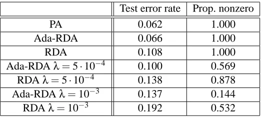
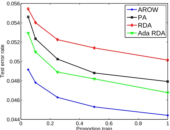
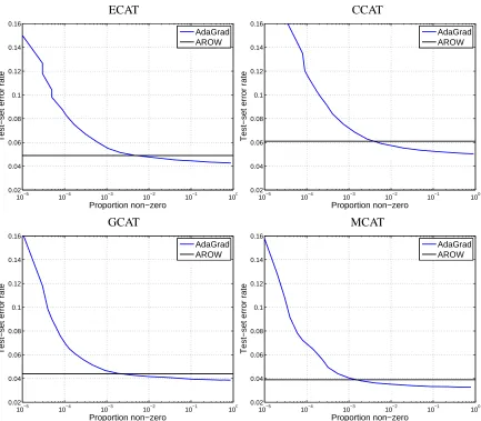
As mentioned in the prequel, we expect our adaptive methods to outperform standard online learning methods when the gradient vectors are sparse. We give empirical evidence supporting the improved performance of the adaptive methods in Section 6. Here we give a few abstract examples that show that for sparse data (input sequences where gt has many zeros) the adaptive methods herein have

better performance than non-adaptive methods. In our examples we use the hinge loss, that is,

ft(x) = [1−ythzt,xi]+ ,

where yt is the label of example t and zt ∈Rdis the data vector.

For our first example, which was also given by McMahan and Streeter (2010), consider the following sparse random data scenario, where the vectors zt ∈ {−1,0,1}d. Assume that at in each

round t, feature i appears with probability pi=min{1,ci−α}for someα∈(1,∞)and a

dimension-independent constant c. Then taking the expectation of the gradient terms in the bound in Corol-lary 1, we have

E

d

∑

i=1

kg1:T,ik₂= d

∑

i=1 E

_q

|{t :_|gt,i|=1}|

≤ d

∑

i=1

q

E|{t :_|gt,i|=1}|= d

∑

i=1

p

piT

by Jensen’s inequality. In the rightmost sum, we have c∑d_i=1i−α/2 =O(log d) for α _≥2, and

∑d

2003) suffers significantly higher loss. We assume the domain

X

gradient descent we setηt=η/√t, which gives the optimal O( √

T)regret (the setting ofηdoes not matter to the adversary we construct).

1.3.1 DIAGONALADAPTATION

Consider the diagonal version of our proposed update (4) with

X

∞≤1}. Evidently, we can take D_∞=2, and this choice simply results in the update xt+1 =xt−

√

2 diag(Gt)−1/2gt

followed by projection (1) onto

X

exist). Let eidenote the ith unit basis vector, and assume that for each t, zt =±ei for some i. Also

let yt=sign(h1,zti)so that there exists a perfect classifier x∗=1∈

X

t =e1. After these

rounds, simply choose zt =±eifor index i∈ {2, . . . ,d}chosen at random. It is clear that the update

to parameter xiat these iterations is different, and amounts to

xt+1=xt+ei ADAGRAD xt+1=

xt+ η √

t

[−1,1]d

(Gradient Descent).

(Here[_·]_[−1,1]d denotes the truncation of the vector to[−1,1]d). In particular, after suffering d−1 more losses, ADAGRAD has a perfect classifier. However, on the remaining iterations gradient descent has η/√t_≤ε and thus evidently suffers loss at least d/(2ε). Of course, for small ε, we have d/(2ε)_≫d. In short, ADAGRADachieves constant regret per dimension while online gradient descent can suffer arbitrary loss (for unbounded t). It seems quite silly, then, to use a global learning rate rather than one for each feature.

Full Matrix Adaptation. We use a similar construction to the diagonal case to show a situation in which the full matrix update from (5) gives substantially lower regret than stochastic gradient descent. For full divergences we set

X

2≤

√

d_}. Let V = [v1 . . . vd]∈Rd×d be an orthonormal matrix. Instead of having zt cycle through the unit vectors, we make zt cycle through

the vi so that zt =±vi. We let the label yt =sign(

1,V⊤zt

) =sign ∑d_i=1hvi,zti

. We provide an elaborated explanation in Appendix A. Intuitively, with ψt(x) =hx,Htxiand Ht set to be the full

matrix from (5), ADAGRAD again needs to observe each orthonormal vector vi only once while

stochastic gradient descent’s loss can be madeΩ(d/ε)for anyε>0.

1.4 Related Work

Many successful algorithms have been developed over the past few years to minimize regret in the online learning setting. A modern view of these algorithms casts the problem as the task of following the (regularized) leader (see Rakhlin, 2009, and the references therein) or FTRL in short. Informally, FTRL methods choose the best decision in hindsight at every iteration. Verbatim usage of the FTRL approach fails to achieve low regret, however, adding a proximal1 term to the past predictions leads to numerous low regret algorithms (Kalai and Vempala, 2003; Hazan and Kale, 2008; Rakhlin, 2009). The proximal term strongly affects the performance of the learning algorithm. Therefore, adapting the proximal function to the characteristics of the problem at hand is desirable. Our approach is thus motivated by two goals. The first is to generalize the agnostic online learn-ing paradigm to the meta-task of specializlearn-ing an algorithm to fit a particular data set. Specifically,

we change the proximal function to achieve performance guarantees which are competitive with the best proximal term found in hindsight. The second, as alluded to earlier, is to automatically adjust the learning rates for online learning and stochastic gradient descent on a per-feature basis. The latter can be very useful when our gradient vectors gt are sparse, for example, in a classification

setting where examples may have only a small number of non-zero features. As we demonstrated in the examples above, it is rather deficient to employ exactly the same learning rate for a feature seen hundreds of times and for a feature seen only once or twice.

Our techniques stem from a variety of research directions, and as a byproduct we also extend a few well-known algorithms. In particular, we consider variants of the follow-the-regularized leader (FTRL) algorithms mentioned above, which are kin to Zinkevich’s lazy projection algorithm. We use Xiao’s recently analyzed regularized dual averaging (RDA) algorithm (2010), which builds upon Nesterov’s (2009) primal-dual subgradient method. We also consider forward-backward splitting (FOBOS) (Duchi and Singer, 2009) and its composite mirror-descent (proximal gradient) general-izations (Tseng, 2008; Duchi et al., 2010), which in turn include as special cases projected gradients (Zinkevich, 2003) and mirror descent (Nemirovski and Yudin, 1983; Beck and Teboulle, 2003). Re-cent work by several authors (Nemirovski et al., 2009; Juditsky et al., 2008; Lan, 2010; Xiao, 2010) considered efficient and robust methods for stochastic optimization, especially in the case when the expected objective f is smooth. It may be interesting to investigate adaptive metric approaches in smooth stochastic optimization.

The idea of adapting first order optimization methods is by no means new and can be traced back at least to the 1970s with the work on space dilation methods of Shor (1972) and variable metric methods, such as the BFGS family of algorithms (e.g., Fletcher, 1970). This prior work often assumed that the function to be minimized was differentiable and, to our knowledge, did not consider stochastic, online, or composite optimization. In her thesis, Nedi´c (2002) studied variable metric subgradient methods, though it seems difficult to derive explicit rates of convergence from the results there, and the algorithms apply only when the constraint set

X

et al. (2009) proposed a Quasi-Newton stochastic gradient-descent procedure, which is similar in spirit to our methods. However, their convergence results assume a smooth objective with positive definite Hessian bounded away from 0. Our results apply more generally.

Prior to the analysis presented in this paper for online and stochastic optimization, the strongly convex functionψin the update equations (3) and (4) either remained intact or was simply multiplied by a time-dependent scalar throughout the run of the algorithm. Zinkevich’s projected gradient, for example, usesψt(x) =kxk2₂, while RDA (Xiao, 2010) employs ψt(x) =√tψ(x) whereψ is a

strongly convex function. The bounds for both types of algorithms are similar, and both rely on the norm_k·k(and its associated dual_k·k∗) with respect to whichψis strongly convex. Mirror-descent type first order algorithms, such as projected gradient methods, attain regret bounds of the form (Zinkevich, 2003; Bartlett et al., 2007; Duchi et al., 2010)

R_φ(T)_≤ 1

ηBψ(x∗,x1) +

η

2

T

∑

t=1

f_t′(x_t)

2

∗ . (7)

Choosingη ∝1/√T gives R_φ(T) =O(√T). When B_ψ(x,x∗)is bounded for all x_∈

X

step sizesηt ∝1/√t which is equivalent to settingψt(x) =√tψ(x). Therefore, no assumption on

(Xiao, 2010, Theorem 3):

Rφ(T)_≤√Tψ(x∗) + 1

2√T

T

∑

t=1

f_t′(x_t)

2

∗ . (8)

The problem of adapting to data and obtaining tighter data-dependent bounds for algorithms such as those above is a natural one and has been studied in the mistake-bound setting for online learning in the past. A framework that is somewhat related to ours is the confidence weighted learning scheme by Crammer et al. (2008) and the adaptive regularization of weights algorithm (AROW) of Crammer et al. (2009). These papers provide mistake-bound analyses for second-order algorithms, which in turn are similar in spirit to the second-second-order Perceptron algorithm (Cesa-Bianchi et al., 2005). The analyses by Crammer and colleagues, however, yield mistake bounds dependent on the runs of the individual algorithms and are thus difficult to compare with our regret bounds.

AROW maintains a mean prediction vector µt∈Rd and a covariance matrixΣt ∈Rd×dover µt

as well. At every step of the algorithm, the learner receives a pair(zt,yt)where zt ∈Rd is the tth

example and yt ∈ {−1,+1}is the label. Whenever the predictor µt attains a margin value smaller

than 1, AROW performs the update

βt =

1

hzt,Σtzti+λ

, αt= [1−ythzt,µti]+,

µt+1=µt+αtΣtytzt, Σt+1=Σt−βtΣtxtx⊤t Σt. (9)

In the above scheme, one can force Σt to be diagonal, which reduces the run-time and storage

requirements of the algorithm but still gives good performance (Crammer et al., 2009). In contrast to AROW, the ADAGRADalgorithm uses the root of the inverse covariance matrix, a consequence of our formal analysis. Crammer et al.’s algorithm and our algorithms have similar run times, generally linear in the dimension d, when using diagonal matrices. However, when using full matrices the runtime of AROW algorithm is O(d2), which is faster than ours as it requires computing the root of a matrix.

In concurrent work, McMahan and Streeter (2010) propose and analyze an algorithm which is very similar to some of the algorithms presented in this paper. Our analysis builds on recent advances in online learning and stochastic optimization (Duchi et al., 2010; Xiao, 2010), whereas McMahan and Streeter use first-principles to derive their regret bounds. As a consequence of our approach, we are able to apply our analysis to algorithms for composite minimization with a known additional objective termϕ. We are also able to generalize and analyze both the mirror descent and dual-averaging family of algorithms. McMahan and Streeter focus on what they term the compet-itive ratio, which is the ratio of the worst case regret of the adaptive algorithm to the worst case regret of a non-adaptive algorithm with the best proximal termψchosen in hindsight. We touch on this issue briefly in the sequel, but refer the interested reader to McMahan and Streeter (2010) for this alternative elegant perspective. We believe that both analyses shed insights into the problems studied in this paper and complement each other.

There are also other lines of work on adaptive gradient methods that are not directly related to our work but nonetheless relevant. Tighter regret bounds using the variation of the cost functions ft

both strongly and weakly convex functions. Our approach differs from previous approaches as it does not focus on a particular loss function or mistake bound. Instead, we view the problem of adapting the proximal function as a meta-learning problem. We then obtain a bound comparable to the bound obtained using the best proximal function chosen in hindsight.

2. Adaptive Proximal Functions

Examining the bounds (7) and (8), we see that most of the regret depends on dual norms of f_t′(xt),

and the dual norms in turn depend on the choice ofψ. This naturally leads to the question of whether we can modify the proximal termψalong the run of the algorithm in order to lower the contribution of the aforementioned norms. We achieve this goal by keeping second order information about the sequence ft and allowψto vary on each round of the algorithms.

We begin by providing two corollaries based on previous work that give the regret of our base algorithms when the proximal function ψt is allowed to change. These corollaries are used in

the sequel in our regret analysis. We assume that ψt is monotonically non-decreasing, that is, ψt+1(x)≥ψt(x). We also assume that ψt is 1-strongly convex with respect to a time-dependent

semi-normk·kψt. Formally,ψis 1-strongly convex with respect tok·kψif

ψ(y)_≥ψ(x) +_h∇ψ(x),y₋x_i+1

2kx−yk 2 ψ .

Strong convexity is guaranteed if and only if B_ψt(x,y)≥ 1

2kx−yk 2

ψt. We also denote the dual norm of_k·kψ

t byk·kψt∗. For completeness, we provide the proofs of following two results in Appendix F, as they build straightforwardly on work by Duchi et al. (2010) and Xiao (2010). For the primal-dual subgradient update, the following bound holds.

Proposition 2 Let the sequence{xt}be defined by the update (3). For any x∗∈

X

∑

t=1

ft(xt) +ϕ(xt)−ft(x∗)−ϕ(x∗)≤

1

ηψT(x∗) + η

2

T

∑

t=1

f_t′(x_t)

2 ψ∗

t−1 . (10)

For composite mirror descent algorithms a similar result holds.

Proposition 3 Let the sequence_{xt}be defined by the update (4). Assume w.l.o.g. thatϕ(x1) =0. For any x∗_∈

X

T

∑

t=1

ft(xt) +ϕ(xt)−ft(x∗)−ϕ(x∗)

≤ 1_ηB_ψ1(x∗,x1) +

1

η T−1

∑

t=1

B_ψt+1(x∗,xt+1)−Bψt(x∗,xt+1)

+η

2

T

∑

t=1

f_t′(x_t)

2 ψ∗

t . (11)

INPUT:η>0,δ_≥0

VARIABLES: s_∈Rd,H_∈Rd×d, g1:t,i∈Rt for i∈ {1, . . . ,d}

INITIALIZEx1=0, g1:0= [] FORt=1 to T

Suffer loss ft(xt)

Receive subgradient gt ∈∂ft(xt)of ft at xt

UPDATEg1:t= [g1:t−1gt], st,i=kg1:t,ik₂

SETHt =δI+diag(st),ψt(x) =1₂hx,Htxi

Primal-Dual Subgradient Update (3):

xt+1=argmin

x∈X

(

η

*

1 t

t

∑

τ=1 g_τ,x

+

+ηϕ(x) +1

tψt(x)

)

.

Composite Mirror Descent Update (4): xt+1=argmin

x∈X

η

hgt,xi+ηϕ(x) +Bψt(x,xt) .

Figure 1: ADAGRADwith diagonal matrices

3. Diagonal Matrix Proximal Functions

We begin by restricting ourselves to using diagonal matrices to define matrix proximal functions and (semi)norms. This restriction serves a two-fold purpose. First, the analysis for the general case is somewhat complicated and thus the analysis of the diagonal restriction serves as a proxy for better understanding. Second, in problems with high dimension where we expect this type of modification to help, maintaining more complicated proximal functions is likely to be prohibitively expensive. Whereas earlier analysis requires a learning rate to slow changes between predictors xt and xt+1, we

will instead automatically grow the proximal function we use to achieve asymptotically low regret. To remind the reader, g1:t,i is the ith row of the matrix obtained by concatenating the subgradients

from iteration 1 through t in the online algorithm.

To provide some intuition for the algorithm we show in Algorithm 1, let us examine the problem

min

s T

∑

t=1

d

∑

i=1 g2_t,i

si

s.t.s0, _h1,s_{i ≤}c.

This problem is solved by setting si=kg1:T,ik2and scaling s so thaths,1i=c. To see this, we can write the Lagrangian of the minimization problem by introducing multipliersλ0 andθ_≥0 to get

L

∑

i=1

kg1:T,ik22 si − h

λ,s_i+θ(_h1,s_{i −}c).

Taking partial derivatives to find the infimum of

L

2/s2i −λi+θ=0, and

com-plementarity conditions onλisi (Boyd and Vandenberghe, 2004) imply thatλi =0. Thus we have

si=θ− 1

2kg_1:T,ik

2, and normalizing appropriately usingθgives that si=ckg1:T,ik2/∑

d j=1

g_1:T,j

As a final note, we can plug siinto the objective above to see inf s ( T

∑

t=1

d

∑

i=1 g2_t,i

si

: s0,_h1,s_{i ≤}c

) =1 c d

∑

kg1:T,ik₂ !2

. (12)

Let diag(v)denote the diagonal matrix with diagonal v. It is natural to suspect that for s achieving the infimum in Equation (12), if we use a proximal function similar toψ(x) =_hx,diag(s)x_i with associated squared dual norm _kx_k2_ψ∗ =

x,diag(s)−1_x

, we should do well lowering the gradient terms in the regret bounds (10) and (11).

To prove a regret bound for our Algorithm 1, we note that both types of updates suffer losses that include a term depending solely on the gradients obtained along their run. The following lemma is applicable to both updates, and was originally proved by Auer and Gentile (2000), though we provide a proof in Appendix C. McMahan and Streeter (2010) also give an identical lemma.

Lemma 4 Let gt= ft′(xt)and g1:t and st be defined as in Algorithm 1. Then T

∑

t=1

gt,diag(st)−1gt

≤2

d

∑

i=1

kg1:T,ik₂ .

To obtain a regret bound, we need to consider the terms consisting of the dual-norm of the sub-gradient in the regret bounds (10) and (11), which iskf_t′(xt)k2_ψ∗

t. Whenψt(x) =hx,(δI+diag(st))xi, it is easy to see that the associated dual-norm is

kg_k2_ψ∗

t =

g,(δI+diag(st))−1g

.

From the definition of st in Algorithm 1, we clearly havekft′(xt)k2_ψ∗

t ≤

gt,diag(st)−1gt

. Note that if st,i=0 then gt,i=0 by definition of st,i. Thus, for anyδ≥0, Lemma 4 implies

T

∑

t=1

f_t′(x_t)

2 ψ∗

t ≤2

d

∑

i=1

kg1:T,ik2. (13)

To obtain a bound for a primal-dual subgradient method, we set δ_≥maxtkgtk_∞, in which case kgtk2_ψ∗

t−1 ≤

gt,diag(st)−1gt

, and we follow the same lines of reasoning to achieve the inequal-ity (13).

It remains to bound the various Bregman divergence terms for Corollary 3 and the termψT(x∗)

for Corollary 2. We focus first on the composite mirror-descent update. Examining the bound (11) and Algorithm 1, we notice that

Bψt+1(x∗,xt+1)−Bψt(x∗,xt+1) = 1 2hx

∗_−x

t+1,diag(st+1−st)(x∗−xt+1)i

≤1₂max

i (x ∗

i −xt+1,i)2kst+1−stk1. Since_kst+1−stk1=hst+1−st,1iandhsT,1i=∑di=1kg1:T,ik₂, we have

T₋1

∑

t=1

B_ψt+1(x∗,xt+1)−Bψt(x∗,xt+1) ≤ 1 2

T₋1

∑

t=1

kx∗₋xt+1k2_∞hst+1−st,1i

≤ 1₂max

t_≤T kx ∗_−x

tk2_∞ d

∑

i=1

kg1:T,ik₂−

1 2kx

∗_−x

We also have

ψT(x∗) =δkx∗k22+hx∗,diag(sT)x∗i ≤δkx∗k22+kx∗k 2 ∞

d

∑

i=1

kg1:T,ik₂.

Combining the above arguments with Corollaries 2 and 3, and using (14) with the fact that B_ψ1(x∗,x1)≤

1

2kx∗−x1k 2

∞h1,s1i, we have proved the following theorem.

Theorem 5 Let the sequence_{xt}be defined by Algorithm 1. For xt generated using the

primal-dual subgradient update (3) withδ≥maxtkgtk_∞, for any x∗∈

X

Rφ(T)_≤ δ

ηkx∗k22+ 1

ηkx∗k2∞

d

∑

i=1

kg1:T,ik₂+η

d

∑

i=1

kg1:T,ik₂.

For xt generated using the composite mirror-descent update (4), for any x∗∈

X

R_φ(T)_≤ 1

2ηmaxt≤T kx ∗_−x

tk2_∞ d

∑

i=1

kg1:T,ik₂+η

d

∑

i=1

kg1:T,ik₂.

The above theorem is a bit unwieldy. We thus perform a few algebraic simplifications to get the next corollary, which has a more intuitive form. Let us assume that

X

sup_x∈Xkx−x∗k∞. Furthermore, define

γT ,

d

∑

i=1

kg1:T,ik₂=inf s

( _T

∑

t=1

gt,diag(s)−1gt

:_h1,s_{i ≤}

d

∑

i=1

kg1:T,ik₂, s0

)

.

Also w.l.o.g. let 0_∈

X

though we have moved the√d term in the earlier bound).

Corollary 6 Assume that D_∞andγT are defined as above. For{xt}generated by Algorithm 1 using the primal-dual subgradient update (3) withη=_kx∗_k∞, for any x∗_∈

X

Rφ(T)_≤2kx∗k∞γT+δ

kx∗k22

kx∗_k∞ ≤2kx

∗_k

∞γT+δkx∗k1 .

Using the composite mirror descent update (4) to generate{xt}and settingη=D∞/√2, we have

R_φ(T)_≤√2D_∞

d

∑

i=1

kg1:T,ik₂= √

2D_∞γT .

We now give a short derivation of Corollary 1 from the introduction: use Theorem 5, Corollary 6, and the fact that

inf s ( T

∑

∑

si

: s0,_h1,s_{i ≤}d

) = 1 d d

∑

kg1:T,ik₂ !2

.

as in (12) in the beginning of Section 3. Plugging theγT term in from Corollary 6 and multiplying

As discussed in the introduction, Algorithm 1 should have lower regret than non-adaptive algo-rithms on sparse data, though this depends on the geometry of the underlying optimization space

X

Then the gradient terms are likewise based on 0/1-valued features and sparse, so the gradient terms in the bound∑d_i=1kg1:T,ik₂should all be much smaller than

√

T . If some features appear much more frequently than others, then the infimal representation ofγT and the infimal equality in Corollary 1

show that we have significantly lower regret by using higher learning rates for infrequent features and lower learning rates on commonly appearing features. Further, if the optimal predictor is rela-tively dense, as is often the case in predictions problems with sparse inputs, then_kx∗_k∞is the best p-norm we can have in the regret.

More precisely, McMahan and Streeter (2010) show that if

X

of radius R and contains anℓ_∞ball of radius r, then the bound in the above corollary is within a factor of √2R/r of the regret of the best diagonal proximal matrix, chosen in hindsight. So, for example, if

X

X

the guarantees we can give on optimality of ADAGRAD.

4. Full Matrix Proximal Functions

In this section we derive and analyze new updates when we estimate a full matrix for the divergence

ψtinstead of a diagonal one. In this generalized case, we use the root of the matrix of outer products

of the gradients that we have observed to update our parameters. As in the diagonal case, we build on intuition garnered from an optimization problem, and in particular, we seek a matrix S which is the solution to the following minimization problem:

min

S T

∑

t=1

gt,S−1gt

s.t.S0, tr(S)_≤c. (15)

The solution is obtained by defining Gt =∑t_τ=1gτgτ⊤ and setting S to be a normalized version of the root of GT, that is, S=c G1_T/2/tr(G1_T/2). For a proof, see Lemma 15 in Appendix E, which also

shows that when GT is not full rank we can instead use its pseudo-inverse. If we iteratively use

divergences of the formψt(x) =

D

x,G1_t/2xE, we might expect as in the diagonal case to attain low regret by collecting gradient information. We achieve our low regret goal by employing a similar doubling lemma to Lemma 4 and bounding the gradient norm terms. The resulting algorithm is given in Algorithm 2, and the next theorem provides a quantitative analysis of the brief motivation above.

Theorem 7 Let Gt be the outer product matrix defined above and the sequence{xt}be defined by

Algorithm 2. For xt generated using the primal-dual subgradient update of (3) andδ≥maxtkgtk2, for any x∗_∈

X

R_φ(T)_≤ δ

ηkx∗k22+ 1

ηkx∗k22tr(G 1/2

T ) +ηtr(G

1/2

T ).

For xt generated with the composite mirror-descent update of (4), if x∗∈

X

Rφ(T)_≤ δ

ηkx∗k22+ 1

2ηmaxt≤T kx ∗_−x

tk22tr(G 1/2

T ) +ηtr(G

1/2

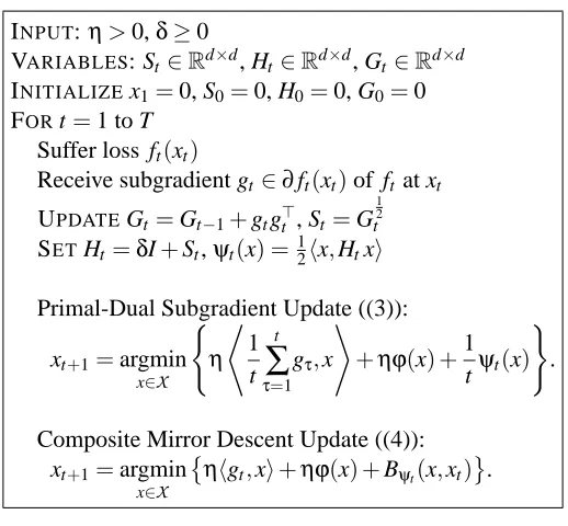
INPUT:η>0,δ_≥0

VARIABLES: St ∈Rd×d, Ht ∈Rd×d, Gt ∈Rd×d

INITIALIZEx1=0, S0=0, H0=0, G0=0 FORt=1 to T

Suffer loss ft(xt)

Receive subgradient gt ∈∂ft(xt)of ft at xt

UPDATEGt =Gt−1+gtg⊤t , St =G 1 2 t

SETHt=δI+St,ψt(x) =1₂hx,Htxi

Primal-Dual Subgradient Update ((3)):

xt+1=argmin

x∈X

(

η

*

1 t

t

∑

τ=1 gτ,x

+

+ηϕ(x) +1

tψt(x)

)

.

Composite Mirror Descent Update ((4)): xt+1=argmin

x_∈X

ηhgt,xi+ηϕ(x) +Bψt(x,xt) .

Figure 2: ADAGRADwith full matrices

Proof To begin, we consider the difference between the divergence terms at time t+1 and time t from the regret (11) in Corollary 3. Letλmax(M)denote the largest eigenvalue of a matrix M. We have

B_ψt+1(x∗,xt+1)−Bψt(x∗,xt+1) = 1 2

D

x∗₋xt+1,(Gt+11/2−Gt1/2)(x∗−xt+1)

E

≤ 1₂kx∗₋xt+1k22λmax(G 1/2

t+1−G 1/2

t ) ≤

1 2kx

∗_−x

t+1k22tr(G 1/2

t+1−G 1/2

t ).

For the last inequality we used the fact that the trace of a matrix is equal to the sum of its eigenvalues along with the property Gt+11/2−Gt1/20 (see Lemma 13 in Appendix B) and therefore tr(G_t+1/21− G1t/2)≥λmax(G1_t+/21−G

1/2

t ). Thus, we get

T₋1

∑

t=1

Bψt+1(x∗,xt+1)−Bψt(x∗,xt+1)≤ 1 2

T₋1

∑

t=1

kx∗₋xt+1k22

tr(G1_t+/2₁)₋tr(G1t/2)

.

Now we use the fact that G1is a rank 1 PSD matrix with non-negative trace to see that

T−1

∑

t=1

kx∗₋xt+1k22

tr(G1_t+/2₁)₋tr(G1t/2)

≤max

t≤T kx ∗_−x

tk22tr(GT1/2)− kx∗−x1k22tr(G 1/2

1 ). (16)

It remains to bound the gradient terms common to all our bounds. We use the following three lemmas, which essentially directly applicable. We prove the first two in Appendix D.

Lemma 8 Let B0 and B−1/2 denote the root of the inverse of B when B≻0 and the root of the pseudo-inverse of B otherwise. For anyνsuch that B₋νgg⊤0 the following inequality holds.

Lemma 9 Letδ_{≥ k}g_k2and A0, theng,(δI+A1/2)−1_g

≤Dg, (A+gg⊤)†1/2

g

E

.

Lemma 10 Let St =Gt1/2 be as defined in Algorithm 2 and A† denote the pseudo-inverse of A.

Then

T

∑

t=1

D

gt,S†tgt

E ≤2 T

∑

gt,S†Tgt

E

=2 tr(GT1/2).

Proof We prove the lemma by induction. The base case is immediate, since we have

D

g1,(G†1) 1/2_g

1

E

=hg1,g1i kg1k2

=_kg1k2≤2kg1k2.

Now, assume the lemma is true for T₋1, so from the inductive assumption we get

T

∑

t=1

D

gt,S†tgt

E

≤2

T−1

∑

t=1

D

gt,S†T−1gt

E

+DgT,S†TgT

E

.

Since ST−1does not depend on t we can rewrite∑Tt=−11

D

gt,S†T−1gt

E

as

tr S†_T−1,

T₋1

∑

t=1 gtg⊤t

!

=tr((G†_T−1)1/2GT₋1),

where the right-most equality follows from the definitions of St and Gt. Therefore, we get

T

∑

t=1

D

gt,S†tgt

E

≤ 2 tr((G†_T−1)1/2GT−1) +

D

gT,(G†T)

1/2_g

T

E

= 2 tr(G1_T/₋2₁) +DgT,(G†T)1/2gT

E

.

Using Lemma 8 with the substitution B=GT,ν=1, and g=gt lets us exploit the concavity of the

function tr(A1/2)to bound the above sum by 2 tr(G1_T/2). N We can now finalize our proof of the theorem. As in the diagonal case, we have that the squared dual norm (seminorm whenδ=0) associated withψt is

kx_k2_ψ∗

t =

x,(δI+St)−1x

.

Thus it is clear that_kgtk2_ψ∗

t ≤

D

gt,St†gt

E

. For the dual-averaging algorithms, we use Lemma 9 above

show that_kgtk2_ψ∗

t−1≤

D

gt,St†gt

E

so long asδ_{≥ k}gtk2. Lemma 10’s doubling inequality then implies that

T

∑

t=1

f_t′(x_t)

2 ψ∗

t ≤2 tr(G 1/2

T ) and

T

∑

t=1

f_t′(x_t)

2 ψ∗

t−1 ≤

2 tr(G1_T/2) (17) for the mirror-descent and primal-dual subgradient algorithm, respectively.

To finish the proof, Note that Bψ1(x∗,x1)≤

1

2kx∗−x1k 2 2tr(G

1/2

1 )whenδ=0. By combining this with the first of the bounds (17) and the bound (16) on∑T_t=−₁1Bψt+1(x∗,x

t+1_)−B ψt(x∗,x

fact that∑T_t=1kf_t′(xt)k2_ψ∗

t−1 ≤2 tr(G

1/2

T )and the bound (16) with Corollary 2 gives the desired bound

on Rφ(T)for the primal-dual subgradient algorithms, which completes the proof of the theorem. As before, we can give a corollary that simplifies the bound implied by Theorem 7. The infimal equality in the corollary uses Lemma 15 in Appendix B. The corollary underscores that for learn-ing problems in which there is a rotation U of the space for which the gradient vectors gt have

small inner productshgt,U gti(essentially a sparse basis for the gt) then using full-matrix proximal

functions can attain significantly lower regret.

Corollary 11 Assume thatϕ(x1) =0. Then the regret of the sequence{xt}generated by Algorithm 2

when using the primal-dual subgradient update withη=_kx∗_k2is R_φ(T)_≤2_kx∗_k2tr(G1_T/2) +δ_kx∗_k2 .

Let

X

x∈Xkx−x∗k₂≤D. Taking η=D/

√

2 and using the composite mirror descent update withδ=0, we have

R_φ(T)_≤√2D tr(G1_T/2) =√2dD

v u u

tinf

S

(

T

∑

t=1

g⊤_t S−1_g

t : S0,tr(S)≤d

)

.

5. Derived Algorithms

In this section, we derive updates using concrete regularization functions ϕ and settings of the domain

X

with the diagonal matrix version of the algorithms we have presented. We focus on the diagonal case for two reasons. First, the updates often take closed-form in this case and carry some intuition. Second, the diagonal case is feasible to implement in very high dimensions, whereas the full matrix version is likely to be confined to a few thousand dimensions. We also discuss how to efficiently compute the updates when the gradient vectors are sparse.

We begin by noting a simple but useful fact. Let Gt denote either the outer product matrix of

gradients or its diagonal counterpart and let Ht =δI+G1t/2, as usual. Simple algebraic

manipula-tions yield that each of the updates (3) and (4) in the prequel can be written in the following form (omitting the stepsizeη):

xt+1=argmin

x∈X

hu,xi+ϕ(x) +1

2hx,Htxi

. (18)

In particular, at time t for the RDA update, we have u=ηt ¯gt. For the composite gradient update (4),

ηhgt,xi+

1

2hx−xt,Ht(x−xt)i=hηgt−Htxt,xi+ 1

2hx,Htxi+ 1

2hxt,Htxti

so that u=ηgt−Htxt. We now derive algorithms for solving the general update (18). Since most

5.1 ℓ1-regularization

We begin by considering how to solve the minimization problems necessary for Algorithm 1 with diagonal matrix divergences and ϕ(x) =λ_kx_k1. We consider the two updates we proposed and denote the ith diagonal element of the matrix Ht =δI+diag(st) from Algorithm 1 by Ht,ii=δ+ kg1:t,ik₂. For the primal-dual subgradient update, the solution to (3) amounts to the following simple

update for xt+1,i:

xt+1,i=sign(−g¯t,i) ηt Ht,ii

[_|g¯t,i| −λ]₊ . (19)

Comparing the update (19) to the standard dual averaging update (Xiao, 2010), which is

xt+1,i=sign(−g¯t,i)η √

t[_|g¯t,i| −λ]₊ ,

it is clear that the difference distills to the step size employed for each coordinate. Our generalization of RDA yields a dedicated step size for each coordinate inversely proportional to the time-based norm of the coordinate in the sequence of gradients. Due to the normalization by this term the step size scales linearly with t, so when Ht,ii is small, gradient information on coordinate i is quickly

incorporated.

The composite mirror-descent update (4) has a similar form that essentially amounts to iterative shrinkage and thresholding, where the shrinkage differs per coordinate:

xt+1,i=sign

xt,i− η

Ht,ii

gt,i

xt,i− η

Ht,ii

gt,i

−

λη

Ht,ii

+

.

We compare the actual performance of the newly derived algorithms to previously studied versions in the next section.

For both updates it is clear that we can perform “lazy” computation when the gradient vectors are sparse, a frequently occurring setting when learning for instance from text corpora. Suppose that from time step t0 through t, the ith component of the gradient is 0. Then we can evaluate the above updates on demand since Ht,iiremains intact. For composite mirror-descent, at time t when

xt,i is needed, we update

xt,i=sign(xt0,i)

|xt0,i| − λη

Ht0,ii (t₋t0)

+

.

Even simpler just in time evaluation can be performed for the the primal-dual subgradient update. Here we need to keep an unnormalized version of the average ¯gt. Concretely, we keep track of

ut=t ¯gt=∑t_τ=1gτ=ut−1+gt, then use the update (19):

xt,i=sign(−ut,i) ηt

Ht,ii

|ut,i|

t −λ

+

,

where Ht can clearly be updated lazily in a similar fashion.

5.2 ℓ1-ball Projections

We next consider the setting in whichϕ_≡0 and

X

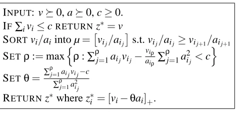
INPUT: v0, a0, c_≥0. IF∑ivi≤cRETURNz∗=v

SORTvi/aiinto µ=

vij/aij

s.t. vij/aij ≥vij+1/aij+1

SETρ:=max

n

ρ:∑ρ_j=1aijvij−

viρ aiρ∑

ρ

j=1a2ij<c

o

SETθ=∑ ρ

j=1ai jvi j−c ∑ρj=1a2_{i j}

RETURNz∗where z∗_i = [vi−θai]₊.

Figure 3: Project v0 to_{z :_ha,z_{i ≤}c,z0_}.

use the matrix Ht =δI+diag(Gt)1/2from Algorithm 1. We provide a brief derivation sketch and

an O(d log d)algorithm in this section. First, we convert the problem (18) into a projection prob-lem onto a scaledℓ1-ball. By making the substitutions z=H1/2x and A=H−1/2, it is clear that problem (18) is equivalent to

min

z

z+H

−1/2_u

2

2 s.t. kAzk1≤c.

Now, by appropriate choice of v=₋H−1/2u=₋ηtHt−1/2g¯t for the primal-dual update (3) and

v=Ht1/2xt−ηHt−1/2gt for the mirror-descent update (4), we arrive at the problem

min

z

1

2kz−vk 2 2 s.t.

d

∑

i=1

ai|zi| ≤c. (20)

We can clearly recover xt+1from the solution z∗to the projection (20) via xt+1=Ht−1/2z∗.

By the symmetry of the objective (20), we can assume without loss of generality that v0 and constrain z0, and a bit of manipulation with the Lagrangian (see Appendix G) for the problem shows that the solution z∗has the form

z∗_i =

vi−θ∗ai if vi≥θ∗ai

0 otherwise

for someθ∗_≥0. The algorithm in Figure 3 constructs the optimalθand returns z∗.

5.3 ℓ2Regularization

We now turn to the case whereϕ(x) =λ_kxk2while

X

min

x hu,xi+

1

2hx,Hxi+λkxk2 . (21) There is no closed form solution for this problem, but we give an efficient bisection-based procedure for solving (21). We start by deriving the dual. Introducing a variable z=x, we get the equivalent problem of minimizing_hu,x_i+1_2hx,Hx_i+λ_kz_k2subject to x=z. With Lagrange multipliersαfor the equality constraint, we obtain the Lagrangian

L

INPUT: u_∈Rd, H0,λ>0. IF_ku_k2≤λ

RETURNx=0

SETv=H−1u,θmax=kvk2/λ−1/σmin(H)

θmin=kvk2/λ−1/σmax(H) WHILEθmax−θmin>ε

SETθ= (θmax+θmin)/2,α(θ) =−(H−1+θI)−1v IF_kα(θ)_k2>λ

SETθmin=θ ELSE

SETθmax=θ

RETURNx=₋H−1(u+α(θ))

Figure 4: Minimize_hu,x_i+1

2hx,Hxi+λkxk2

Taking the infimum of

L

attained at x=₋H−1(u+α). Coupled with the fact that infzλkzk2− hα,zi=−∞unlesskαk2≤λ, in which case the infimum is 0, we arrive at the dual form

inf

x,z

L

−1 2

u+α,H−1(u+α)

if _kα_k2≤λ

−∞ otherwise.

Setting v=H−1u, we further distill the dual to

min

α hv,αi+ 1 2

α

,H−1α

s.t. _kα_k2≤λ. (22) We can solve problem (22) efficiently using a bisection search of its equivalent representation in Lagrange form,

min

α hv,αi+ 1 2

α,H−1α+θ

2kαk 2 2 ,

whereθ>0 is an unknown scalar. The solution to the latter as a function ofθis clearlyα(θ) = −(H−1+θI)−1_v=−(H−1_+θI)−1_H−1_{u. Sincekα(θ)k}

2is monotonically decreasing inθ(consider the the eigen-decomposition of the positive definite H−1_{), we can simply perform a bisection search} overθ, checking at each point whether_kα(θ)_k2≷λ.

To find initial upper and lower bounds onθ, we note that

(1/σmax(H) +θ)−1kvk2≤ kα(θ)k2≤(1/σmin(H) +θ)−1kvk2

whereσmax(H)denotes the maximum singular value of H andσmin(H)the minimum. To guarantee

kα(θmax)k2≤λ, we thus setθmax=kvk2/λ−1/σmax(H). Similarly, forθminwe see that so long as

5.4 ℓ_∞Regularization

We again let

X

∞. This type of update, similarly toℓ2, zeroes groups of variables, which is handy in finding structurally sparse solutions for multitask or multi-class problems. Solving theℓ_∞regularized problem amounts to

min

x hu,xi+

1

2hx,Hxi+λkxk∞ . (23)

The dual of this problem is a modifiedℓ1-projection problem. As in the case ofℓ2regularization, we introduce an equality constrained variable z=x with associated Lagrange multipliersα_∈Rdto obtain

L

2hx,Hxi+λkzk∞+hα,x−zi .

Performing identical manipulations to theℓ2case, we take derivatives and get that x=−H−1(u+α) and, similarly, unless_kα_k1≤λ, infz

L

max α −

1

2(u+α)H

−1_{(u+α) s.t.}

kαk1≤λ.

When H is diagonal we can find the optimalα∗using the generalizedℓ1-projection in Algorithm 3, then reconstruct the optimal x via x=₋H−1(u+α∗_).

5.5 Mixed-norm Regularization

Finally, we combine the above results to show how to solve problems with matrix-valued inputs X _∈Rd×k, where X= [x1 ··· xd]⊤. We consider mixed-norm regularization, which is very useful for encouraging sparsity across several tasks (Obozinski et al., 2007). Nowϕis anℓ1/ℓpnorm, that

is,ϕ(X) =λ∑d

i=1kxikp. By imposing an ℓ1-norm over p-norms of the rows of X , entire rows are

nulled at once.

When p_{∈ {}2,∞_}and the proximal H in (18) is diagonal, the previous algorithms can be readily used to solve the mixed norm problems. We simply maintain diagonal matrix information for each of the rows ¯xi of X separately, then solve one of the previous updates for each row independently.

We use this form of regularization in our experiments with multiclass prediction problems in the next section.

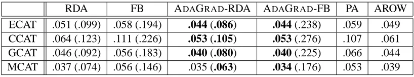
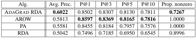
6. Experiments