Faster Algorithms for Max-Product Message-Passing

(1)

Faster Algorithms for Max-Product Message-Passing

∗

Julian J. McAuley† [email protected]

Tib´erio S. Caetano† [email protected] Statistical Machine Learning Group

NICTA

Locked Bag 8001

Canberra ACT 2601, Australia

Editor: Tommi Jaakkola

Abstract

Maximum A Posteriori inference in graphical models is often solved via message-passing

algo-rithms, such as the junction-tree algorithm or loopy belief-propagation. The exact solution to this problem is well-known to be exponential in the size of the maximal cliques of the triangulated model, while approximate inference is typically exponential in the size of the model’s factors. In this paper, we take advantage of the fact that many models have maximal cliques that are larger than their constituent factors, and also of the fact that many factors consist only of latent variables (i.e., they do not depend on an observation). This is a common case in a wide variety of applications that deal with grid-, tree-, and ring-structured models. In such cases, we are able to decrease the exponent of complexity for message-passing by 0.5 for both exact and approximate inference. We demonstrate that message-passing operations in such models are equivalent to some variant of ma-trix multiplication in the tropical semiring, for which we offer an O(N2.5)expected-case solution. Keywords: graphical models, belief-propagation, tropical matrix multiplication

1. Introduction

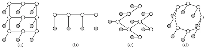
It is well-known that exact inference in tree-structured graphical models can be accomplished ef-ficiently by message-passing operations following a simple protocol making use of the distributive law (Aji and McEliece, 2000; Kschischang et al., 2001). It is also well-known that exact inference in arbitrary graphical models can be solved by the junction-tree algorithm; its efficiency is deter-mined by the size of the maximal cliques after triangulation, a quantity related to the tree-width of the graph.

Figure 1 illustrates an attempt to apply the junction-tree algorithm to some graphical models containing cycles. If the graphs are not chordal ((a) and (b)), they need to be triangulated, or made chordal (red edges in (c) and (d)). Their clique-graphs are then guaranteed to be junction-trees, and the distributive law can be applied with the same protocol used for trees; see Aji and McEliece (2000) for a beautiful tutorial on exact inference in arbitrary graphs. Although the models in these

∗. Preliminary versions of this work appeared in The 27th International Conference on Machine Learning (ICML 2010), and the 13th International Conference on Artificial Intelligence and Statistics (AISTATS 2010), The NIPS 2009 Workshop on Learning with Orderings, The NIPS 2009 Workshop on Discrete Optimization in Machine Learning, and in Learning and Intelligent Optimization (LION 4).

(2)

(a) (b) (c) (d)

Figure 1: The models at left ((a) and (b)) can be triangulated ((c) and (d)) so that the junction-tree algorithm can be applied. Despite the fact that the new models have larger maximal cliques, the corresponding potentials are still factored over pairs of nodes only. Our algorithms exploit this fact.

(a) (b) (c) (d)

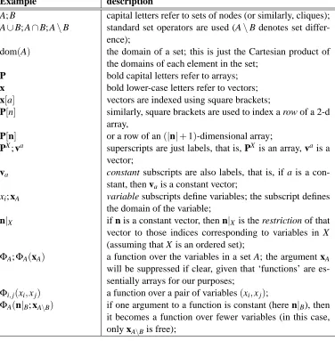
Figure 2: Some graphical models to which our results apply: factors conditioned upon observations

have fewer latent variables than purely latent factors. White nodes correspond to latent

variables, gray nodes to an observation. In other words, factors containing a gray node encode the data likelihood, whereas factors containing only white nodes encode priors. Expressed more simply, the ‘node potentials’ depend upon the observation, while the ‘edge potentials’ do not.

examples contain only pairwise factors, triangulation has increased the size of their maximal cliques, making exact inference substantially more expensive. Hence approximate solutions in the original graph (such as loopy belief-propagation, or inference in a loopy factor-graph) are often preferred over an exact solution via the junction-tree algorithm.

Even when the model’s factors are the same size as its maximal cliques, neither exact nor ap-proximate inference algorithms take advantage of the fact that many factors consist only of latent variables. In many models, those factors that are conditioned upon the observation contain fewer latent variables than the purely latent factors. Examples are shown in Figure 2. This encompasses a wide variety of models, including grid-structured models for optical flow and stereo disparity as well as chain and tree-structured models for text or speech.

In this paper, we exploit the fact that the maximal cliques (after triangulation) often have po-tentials that factor over subcliques, as illustrated in Figure 1. We will show that whenever this is the case, the expected computational complexity of message-passing between such cliques can be

improved (both the asymptotic upper-bound and the actual runtime).

Additionally, we will show that this result can be applied in cliques whose factors that are

(3)

of latent variables; the ‘purely latent’ factors can be pre-processed offline, allowing us to achieve the same benefits as described in the previous paragraph.

We show that these properties reveal themselves in a wide variety of real applications.

A core operation encountered in the junction-tree algorithm is that of computing the inner-product of two vectors va and vb. In the max-product semiring (used for MAP inference), the

‘inner-product’ becomes

max

i∈{1...N}{va[i]×vb[i]}. (1) Our results stem from the realization that while (Equation 1) appears to be a linear time operation, it can be decreased to O(√N)(in the expected case) if we know the permutations that sort vaand vb (i.e., the order statistics of vaand vb). These permutations can be obtained efficiently when the

model factorizes as described above.

Preliminary versions of this work have appeared in McAuley and Caetano (2009), McAuley and Caetano (2010a), and McAuley and Caetano (2010b).

1.1 Summary of Results

A selection of the results to be presented in the remainder of this paper can be summarized as follows:

• Our speedups apply to the operation of passing a single message. As a result, our method can be used regardless of the message-passing protocol.

• We are able to lower the asymptotic expected running time of max-product message-passing for any discrete graphical model whose cliques factorize into lower-order terms.

• The results obtained are exactly those that would be obtained by the traditional version of the algorithm, that is, no approximations are used.

• Our algorithm also applies whenever factors that are conditioned upon an observation contain fewer latent variables than those factors that are not conditioned upon an observation, as in Figure 2 (in which case certain computations can be taken offline).

• For pairwise models satisfying the above properties, we obtain an expected speed-up of at

leastΩ(√N)(assuming N states per node;Ωdenotes an asymptotic lower-bound). For exam-ple, in models with third-order cliques containing pairwise terms, message-passing is reduced fromΘ(N3₎_{to O}₍_N2√_N₎_{, as in Figure 1(d). For pairwise models whose edge potential is not}

conditioned upon an observation, message-passing is reduced fromΘ(N2)to O(N√N), as in Figure 2.

• For cliques composed of K-ary factors, the expected speed-up generalizes to at leastΩ(1 KN

1

K),

though it is never asymptotically slower than the original solution.

• The expected-case improvement is derived under the assumption that the order statistics of different factors are independent.

(4)

• If the different factors have ‘opposite’ order statistics, the performance will be worse than the expected case, but is never asymptotically more expensive than the traditional version of the algorithm.

Our results do not apply for every semiring (_⊕,_⊗), but only to those whose ‘addition’ oper-ation defines an order (for example, min or max); we also assume that under this ordering, our ‘multiplication’ operator_⊗satisfies

a<b_∧c<d _⇒ a_⊗c<b_⊗d. (2) Thus our results certainly apply to the sum and min-sum (‘tropical’) semirings (as well as

max-product and min-max-product, assuming non-negative potentials), but not for sum-max-product (for example).

Consequently, our approach is useful for computing MAP-states, but cannot be used to compute marginal distributions. We also assume that the domain of each node is discrete.

We shall initially present our algorithm in terms of pairwise graphical models such as those shown in Figure 2. In such models message-passing is precisely equivalent to matrix-vector mul-tiplication over our chosen semiring. Later we shall apply our results to models such as those in Figure 1, wherein message-passing becomes some variant of matrix multiplication. Finally we shall explore other applications besides message-passing that make use of tropical matrix multiplication as a subroutine, such all-pairs shortest-path problems.

1.2 Related Work

There has been previous work on speeding-up message-passing algorithms by exploiting different types of structure in certain graphical models. For example, Kersting et al. (2009) study the case where different cliques share the same potential function. In Felzenszwalb and Huttenlocher (2006), fast message-passing algorithms are provided for cases in which the potential of a 2-clique is only dependent on the difference of the latent variables (which is common in some computer vision applications); they also show how the algorithm can be made faster if the graphical model is a bipartite graph. In Kumar and Torr (2006), the authors provide faster algorithms for the case in which the potentials are truncated, whereas in Petersen et al. (2008) the authors offer speed-ups for models that are specifically grid-like.

The latter work is perhaps the most similar in spirit to ours, as it exploits the fact that certain factors can be sorted in order to reduce the search space of a certain maximization problem.

Another course of research aims at speeding-up message-passing algorithms by using ‘informed’ scheduling routines, which may result in faster convergence than the random schedules typically used in loopy belief-propagation and inference in factor graphs (Elidan et al., 2006). This branch of research is orthogonal to our own in the sense that our methods can be applied independently of the choice of message passing protocol.

Another closely related paper is that of Park and Darwiche (2003). This work can be seen to compliment ours in the sense that it exploits essentially the same type of factorization that we study, though it applies to sum-product versions of the algorithm, rather than the max-product version that we shall study. Kjærulff (1998) also exploits factorization within cliques of junction-trees, albeit a different type of factorization than that studied here.

(5)

Example description

A; B capital letters refer to sets of nodes (or similarly, cliques);

A_∪B; A_∩B; A_\B standard set operators are used (A_\B denotes set

differ-ence);

dom(A) the domain of a set; this is just the Cartesian product of the domains of each element in the set;

P bold capital letters refer to arrays;

x bold lower-case letters refer to vectors;

x[a] vectors are indexed using square brackets;

P[n] similarly, square brackets are used to index a row of a 2-d array,

P[n] or a row of an(_|n|+1)-dimensional array;

PX; va superscripts are just labels, that is, PX is an array, vais a vector;

va constant subscripts are also labels, that is, if a is a

con-stant, then vais a constant vector;

xi; xA variable subscripts define variables; the subscript defines

the domain of the variable;

n_|X if n is a constant vector, then n|X is the restriction of that

vector to those indices corresponding to variables in X (assuming that X is an ordered set);

ΦA;ΦA(xA) a function over the variables in a set A; the argument xA

will be suppressed if clear, given that ‘functions’ are es-sentially arrays for our purposes;

Φi,j(xi,xj) a function over a pair of variables(xi,xj);

ΦA(n|B; xA_\B) if one argument to a function is constant (here n|B), then

it becomes a function over fewer variables (in this case, only xA\Bis free);

Table 1: Notation

2. Background

The notation we shall use is briefly defined in Table 1. We shall assume throughout that the

max-product semiring is being used, though our analysis is almost identical for any suitable choice.

MAP-inference in a graphical model

G

consists of solving an optimization problem of the form

ˆx=argmax x _C

∏

_∈_CΦC

(xC),

where

C

is the set of maximal cliques in

G

. This problem is often solved via message-passing algorithms such as the junction-tree algorithm, loopy belief-propagation, or inference in a factor-graph (Aji and McEliece, 2000; Weiss, 2000; Kschischang et al., 2001).

Often, the clique-potentialsΦC(xC)shall be decomposable into several smaller factors, that is,

ΦC(xC) =

∏

F⊆C

(6)

Some simple motivating examples are shown in Figure 3: a model for pose estimation from Sigal and Black (2006), a ‘skip-chain CRF’ from Galley (2006), and a model for shape-matching from Coughlan and Ferreira (2002). In each case, the triangulated model has third-order cliques, but the potentials are only pairwise. Other examples have already been shown in Figure 1; analogous cases are ubiquitous in many real applications.

It will often be more convenient to express our objective function as being conditioned upon some observation, y. Thus our optimization problem becomes

ˆx(y) =argmax x _C

∏

_∈_C

ΦC(xC|y) (3)

(for simplicity when we discuss ‘cliques’ we are referring to sets of latent variables).

Further factorization may be possible if we express (Equation 3) in terms of those factors that depend upon the observation y, and those that do not:

ˆx(y) =argmax x _C

∏

_∈_C

n

∏

F⊆C

ΦF(xF)

| {z }

data-independent

×

∏

Q⊆C

ΦQ(xQ|y)

| {z }

data-dependent

o

,

We shall say that those factors that are not conditioned on the observation are ‘data-independent’. Our results shall apply to message-passing equations in those cliques C where for each data-independent factor F we have F _⊂C, or for each data-dependent factor Q we have Q_⊂C, that

is, when all F or all Q in C are proper subsets of C. In such cases we say that the clique C is

factorizable.

The fundamental step encountered in message-passing algorithms is defined below. The mes-sage from a clique X to an intersecting clique Y (both sets of latent variables) is defined by

mX→Y(xX∩Y) =max

xX\Y

(

ΦX(xX)

∏

Z∈Γ(X)\Y

mZ→X(xX∩Z)

)

(4)

(whereΓ(X)is the set of neighbors of the clique X , that is, the set of cliques that intersect with X ). If such messages are computed after X has received messages from all of its neighbors except Y (i.e.,Γ(X)_\Y ), then this defines precisely the update scheme used by the junction-tree algorithm.

The same update scheme is used for loopy belief-propagation, though it is done iteratively in a randomized fashion.

After all messages have been passed, the MAP-state for a set of latent variables M (assumed to be a subset of a single clique X ) is computed using

mM(xM) =max

xX\M

(

ΦX(xX)

∏

Z∈Γ(X)

mZ→X(xX∩Z)

)

. (5)

For cliques that are factorizable (according to our previous definition), both (Equation 4) and (Equation 5) take the form

mM(xM) =max

xX\M

(

∏

F⊆X

ΦF(xF)

∏

Q⊆X

ΦQ(xQ|y)

)

(7)

(a) (b) (c)

Figure 3: (a) A model for pose reconstruction from Sigal and Black (2006); (b) A ‘skip-chain CRF’ from Galley (2006); (c) A model for deformable matching from Coughlan and Ferreira (2002). Although the (triangulated) models have cliques of size three, their potentials factorize into pairwise terms.

Note that we always have Z_∩X_⊂X for messages Z_→X , meaning that the presence of the messages

has no effect on the ‘factorizability’ of (Equation 6).

Algorithm 1 gives the traditional solution to this problem, which does not exploit the factor-ization ofΦX(xX). This algorithm runs inΘ(N|X|), where N is the number of states per node, and

|X_|is the size of the clique X (for a given xX, we treat computing∏F⊂XΦF(xF)as a constant time

operation, as our optimizations shall not modify this cost).

In the following sections, we shall consider the two types of factorizability separately: first, in Section 3, we shall consider cliques X whose messages take the form

mM(xM) =max

xX\M

(

ΦX(xX)

∏

Q⊂X

ΦQ(xQ|y)

)

.

We say that such cliques are conditionally factorizable (since all conditional terms factorize); ex-amples are shown in Figure 2. Next, in Section 4, we consider cliques whose messages take the form

mM(xM) =max

xX\M_F

∏

_⊂_X

ΦF(xF).

We say that such cliques are latently factorizable (since terms containing only latent variables fac-torize); examples are shown in Figure 1.

3. Optimizing Algorithm 1: Conditionally Factorizable Models

In order to specify a more efficient version of Algorithm 1, we begin by considering the simplest nontrivial conditionally factorizable model: a pairwise model in which each latent variable depends upon the observation, that is,

ˆx(y) =argmax x _i

∏

_∈_NΦi

(xi|y)

| {z }

node potential

×

∏

(i,j)∈E

Φi,j(xi,xj)

| {z }

edge potential

. (7)

(8)

Algorithm 1 Brute-force computation of max-marginals

Input: a clique X whose max-marginal mM(xM)(where M⊂X ) we wish to compute; assume that

each node in X has domain_{1. . .N_} 1: for m_∈dom(M)_{i.e.,_{1. . .N_}|M|_}do 2: max :=₋∞

3: for z_∈dom(X_\M)do

4: if∏_F_⊂_XΦF(m|F; z|F)>max then 5: max :=∏F⊂XΦF(m|F; z|F) 6: end if

7: end for_{this loop takesΘ(N|X\M|)_}

8: mM(m):=max

9: end for_{this loop takesΘ(N|X|)_}

10: Return: mM

Message-passing in models of the type shown in (Equation 7) takes the form

mA→B(xi) =Φi(xi|y)×max xj

Φj(xj|y)×Φi,j(xi,xj) (8)

(where A=_{i,j_} and B=_{i,k_}). Note once again that in (Equation 8) we are not concerned solely with exact inference via the junction-tree algorithm. In many models, such as grids and rings, (Equation 7) shall be solved approximately by means of either loopy belief-propagation, or inference in a factor-graph, which consists of solving (Equation 8) according to protocols other than the optimal junction-tree protocol.

It is useful to consider Φi,j in (Equation 8) as an N×N matrix, and Φj as an N-dimensional vector, so that solving (Equation 8) is precisely equivalent to matrix-vector multiplication in the

max-product semiring. For a particular value xi=q, (Equation 8) becomes

mA→B(q) =Φi(q|y)×max xj

Φj(xj|y)

| {z } va

×Φi,j(q,xj)

| {z } vb

, (9)

which is precisely the ‘max-product inner-product’ operation that we claimed was critical in Section 1.

As we have previously suggested, it will be possible to solve (Equation 9) efficiently if we know the order statistics of va and vb, that is, if we know the permutations that sortΦj and every

row ofΦi,j in (Equation 8). SortingΦj takesΘ(N log N), whereas sorting every row ofΦi,j takes

Θ(N2_{log N}₎₍Θ₍_{N log N}₎_{for each of N rows). The critical point to be made is that}Φ

i,j(xi,xj)does not depend on the observation, meaning that its order statistics can be obtained offline in several

applications.

The following elementary lemma is the key observation required in order to solve (Equation 1), and therefore (Equation 9) efficiently:

(9)

Algorithm 2 Find i such that va[i]×vb[i]is maximized

Input: two vectors va and vb, and permutation functions pa and pb that sort them in decreasing

order (so that va[pa[1]]is the largest element in va)

1: Initialize: start :=1, enda:= pa−1[pb[1]], endb := p−b1[pa[1]] {if endb=k, then the largest

element in vahas the same index as the kthlargest element in vb} 2: best :=pa[1], max :=va[best]×vb[best]

3: if va[pb[1]]×vb[pb[1]]>max then 4: best :=pb[1], max :=va[best]×vb[best] 5: end if

6: while start<enda{in practice, we could also stop if start<endb, but the version given here is

the one used for analysis in Appendix A_}do 7: start :=start+1

8: if va[pa[start]]×vb[pa[start]]>max then 9: best :=pa[start]

10: max :=va[best]×vb[best] 11: end if

12: if p−_b1[pa[start]]<endbthen 13: endb:=p−_b1[pa[start]] 14: end if

15: {repeat lines 8–14, interchanging a and b_}

16: end while{this loop takes expected time O(√N)_}

17: Return: best

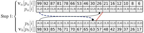
This observation is used to construct Algorithm 2. Here we iterate through the indices starting from the largest values of vaand vb, stopping once both indices are ‘behind’ the maximum value

found so far (which we then know is the maximum). This algorithm is demonstrated pictorially in Figure 4. Note that Lemma 1 only depends upon the relative values of elements in va and vb,

meaning that the number of computations that must be performed is purely a function of their order

statistics (i.e., it does not depend on the actual values of vaor vb).

If Algorithm 2 can solve (Equation 9) in O(f(N)), then we can solve (Equation 8) in O(N f(N)). Determining precisely the running time of Algorithm 2 is not trivial, and will be explored in depth in Appendix A. At this stage we shall state an upper-bound on the true complexity in the following theorem:

Theorem 2 The expected running time of Algorithm 2 is O(√N), yielding a speed-up of at least Ω(√N) in cliques containing pairwise factors. This expectation is derived under the assumption that vaand vbhave independent order statistics.

Algorithm 3 uses Algorithm 2 to solve (Equation 8), where we assume that the order statistics of the rows ofΦi,jhave been obtained offline.

(10)

Step 1:               

6 2 14 16 9 7 12 8 10 3 11 13 1 15 4 5 99 92 87 81 78 66 53 46 30 26 21 16 12 10 8 6

3 4 8 11 7 16 13 9 6 2 15 10 12 5 1 14 98 93 85 76 71 70 67 65 63 57 48 42 39 37 26 17

don't search past this line

Step 2:               

6 2 14 16 9 7 12 8 10 3 11 13 1 15 4 5 99 92 87 81 78 66 53 46 30 26 21 16 12 10 8 6

3 4 8 11 7 16 13 9 6 2 15 10 12 5 1 14 98 93 85 76 71 70 67 65 63 57 48 42 39 37 26 17

Step 3:               

6 2 14 16 9 7 12 8 10 3 11 13 1 15 4 5 99 92 87 81 78 66 53 46 30 26 21 16 12 10 8 6

3 4 8 11 7 16 13 9 6 2 15 10 12 5 1 14 98 93 85 76 71 70 67 65 63 57 48 42 39 37 26 17

Step 4:               

6 2 14 16 9 7 12 8 10 3 11 13 1 15 4 5 99 92 87 81 78 66 53 46 30 26 21 16 12 10 8 6

3 4 8 11 7 16 13 9 6 2 15 10 12 5 1 14 98 93 85 76 71 70 67 65 63 57 48 42 39 37 26 17

Step 5:               

6 2 14 16 9 7 12 8 10 3 11 13 1 15 4 5 99 92 87 81 78 66 53 46 30 26 21 16 12 10 8 6

3 4 8 11 7 16 13 9 6 2 15 10 12 5 1 14 98 93 85 76 71 70 67 65 63 57 48 42 39 37 26 17

Figure 4: Algorithm 2, explained pictorially. The arrows begin at pa[start]and pb[start]; the red

dashed line connects enda and endb, behind which we need not search; a dashed arrow

is used when a new maximum is found. Note that in the event that va and vb contain

repeated elements, they can be sorted arbitrarily.

(11)

Algorithm 3 Solve (Equation 8) using Algorithm 2

Input: a potentialΦi,j(a,b)×Φi(a|yi)×Φj(b|yj)whose max-marginal mi(xi)we wish to compute,

and a set of permutation functions P such that P[i]sorts the ithrow ofΦi,j(in decreasing order). 1: compute the permutation function paby sortingΨj {takesΘ(N log N)}

2: for q_{∈ {}1. . .N_}do

3: (va,vb):= (Ψj,Φi,j(q,xj|yi,yj)) 4: best :=Algorithm2(va,vb,pa,P[q]){O(

√

N)_}

5: mA_→B(q):=Φi(q)×Φj(best)×Φi,j(q,best|yi,yj) 6: end for_{this loop takes expected time O(N√N)_}

7: Return: mA→B

iterations isΩ(log N)), we shall again gain speed improvements even when the sorting step is done online.

In fact, the second of these conditions obviates the need for ‘conditional factorizability’ (or ‘data-independence’) altogether. In other words, in any pairwise model in whichΩ(log N)iterations of belief-propagation are to be performed, the pairwise terms need to be sorted only during the first

iteration. Thus these improvements apply to those models in Figure 1, so long as the number of

iterations of belief-propagation isΩ(log N).

4. Latently Factorizable Models

Just as we considered the simplest conditionally factorizable model in Section 3, we now consider the simplest nontrivial latently factorizable model: a clique of size three containing pairwise factors. In such a case, our aim is to compute

mi,j(xi,xj) =max xk

Φi,j,k(xi,xj,xk), (10)

which we have assumed takes the form

mi,j(xi,xj) =max xk

Φi,j(xi,xj)×Φi,k(xi,xk)×Φj,k(xj,xk).

For a particular value of(xi,xj) = (a,b), we must solve

mi,j(a,b) =Φi,j(a,b)×max xk

Φi,k(a,xk)

| {z } va

×Φj,k(b,xk)

| {z } vb

, (11)

which again is in precisely the form shown in (Equation 1).

Just as (Equation 8) resembled matrix-vector multiplication, there is a close resemblance be-tween (Equation 11) and the problem of matrix-matrix multiplication in the max-product semiring (often referred to as ‘tropical matrix multiplication’, ‘funny matrix multiplication’, or simply ‘max-product matrix multiplication’). While traditional matrix multiplication is well-known to have a subcubic worst-case solution (see Strassen, 1969), the version in (Equation 11) has no known sub-cubic solution (the fastest known solution is O(N3_/_{log N}₎_{, but there is no known solution that runs}

(12)

Algorithm 4 Use Algorithm 2 to compute the max-marginal of a 3-clique containing pairwise

fac-tors

Input: a potential Φi,j,k(a,b,c) = Φi,j(a,b) ×Φi,k(a,c) ×Φj,k(b,c) whose max-marginal mi,j(xi,xj)we wish to compute

1: for n∈ {1. . .N}do

2: compute Pi[n]by sortingΦi,k(n,xk){takesΘ(N log N)}

3: compute Pj[n] by sorting Φj,k(n,xk) {Pi and Pj are N×N arrays, each row of which is

a permutation; Φi,k(n,xk) andΦj,k(n,xk) are functions over xk, since n is constant in this

expression_}

4: end for_{this loop takesΘ(N2log N)_}

5: for(a,b)_{∈ {}1. . .N}2do

6: (va,vb):= Φi,k(a,xk),Φj,k(b,xk)

7: (pa,pb):= Pi[a],Pj[b]

8: best :=Algorithm2(va,vb,pa,pb){takes O(

√

N)_}

9: mi,j(a,b):=Φi,j(a,b)×Φi,k(a,best)×Φj,k(b,best) 10: end for_{this loop takes O(N2√N)_}

{the total running time is O(N2log N+N2√N), which is dominated by O(N2√N)_}

11: Return: mi,j

equivalent to the all-pairs shortest-path problem, which is studied in Alon et al. (1997). Although we shall not improve the worst-case complexity, Algorithm 2 leads to far better expected-case per-formance than existing solutions.

In principle Strassen’s algorithm could be used to perform sum-product inference in the set-ting we discuss here, and indeed there has been some work on performing sum-product infer-ence in graphical models that factorize (Park and Darwiche, 2003). Interestingly, there is also a sub-quadratic solution to sum-product matrix-vector multiplication that requires preprocessing (Williams, 2007), that is, the sum-product version of the setting we discussed in Section 3.

A prescription of how Algorithm 2 can be used to solve (Equation 10) is given in Algorithm 4. As we mentioned in Section 3, the expected-case running time of Algorithm 2 is O(√N), meaning that the time taken to solve Algorithm 4 is O(N2√N).

5. Extensions

So far we have only considered the case of pairwise graphical models, though as mentioned our results can in principle be applied to any conditionally or latently factorizable models, no matter the size of the factors. Essentially our results about matrices become results about tensors. We first treat latently factorizable models, after which the same ideas can be applied to conditionally factorizable models.

5.1 An Extension to Higher-Order Cliques with Three Factors

(13)

Step 1:        

      

(1,2)

99 92 87 81 78 66 53 46 30 26 21 16 12 10 8 6

98 93 85 76 71 70 67 65 63 57 48 42 39 37 26 17 (4,2) (3,2) (4,4) (2,1) (1,3) (3,4) (2,4) (2,2) (4,3) (2,3) (3,1) (4,1) (3,3) (1,4) (1,1)

(4,3) (1,4) (2,4) (2,3) (1,3) (4,4) (3,1) (2,1) (1,2) (4,2) (3,3) (2,2) (3,4) (1,1) (4,1) (3,2)

Figure 5: The reasoning applied in Algorithm 2 applies even when the elements of paand pb are

multidimensional indices.

be adapted to solve

mi,j(xi,xj) =max xk,xm

Φi,j(xi,xj)×Φi,k,m(xi,xk,xm)×Φj,k,m(xj,xk,xm), (12)

and similar variants containing three factors. Here both xkand xmare shared byΦi,k,mandΦj,k,m. We

can follow precisely the reasoning of the previous section, except that when we sortΦi,k,m(similarly

Φj,k,m) for a fixed value of xi, we are now sorting an array rather than a vector (Algorithm 4, lines 2

and 3); in this case, the permutation functions pa and pb in Algorithm 2 simply return pairs of

indices. This is illustrated in Figure 5. Effectively, in this example we are sorting the variable xk,m

whose domain is dom(xk)×dom(xm), which has state space of size N2.

As the number of shared terms increases, so does the improvement to the running time. While (Equation 12) would take Θ(N4) to solve using Algorithm 1, it takes only O(N3) to solve using Algorithm 4 (more precisely, if Algorithm 2 takes O(f(N)), then (Equation 12) takes O(N2f(N2)), which we have mentioned is O(N2√N2_{) =}_O₍_N3₎_{). In general, if we have S shared terms, then the}

running time is O(N2√NS₎_{, yielding a speed-up of}Ω₍√_NS₎_{over the na¨ıve solution of Algorithm 1.} 5.2 An Extension to Higher-Order Cliques with Decompositions Into Three Groups

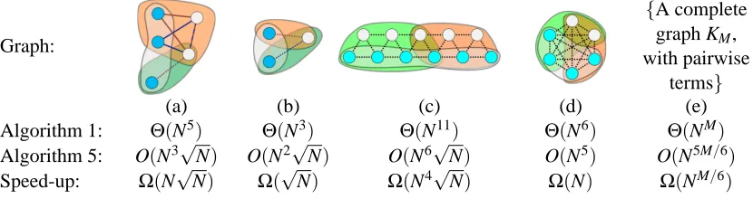
By similar reasoning, we can apply our algorithm to cases where there are more than three factors, in which the factors can be separated into three groups. For example, consider the clique in Figure 6(a), which we shall call G (the entire graph is a clique, but for clarity we only draw an edge when the corresponding nodes belong to a common factor). Each of the factors in this graph have been labeled using either differently colored edges (for factors of size larger than two) or dotted edges (for factors of size two), and the max-marginal we wish to compute has been labeled using colored nodes. We assume that it is possible to split this graph into three groups such that every factor is contained within a single group, along with the max-marginal we wish to compute (Figure 6, (b)). If such a decomposition is not possible, we will have to resort to further extensions to be described in Section 5.3.

Ideally, we would like these groups to have size _{≃ |}G_|/3, though in the worst case they will have size no larger than_|G_{| −}1. We call these groups X , Y , Z, where X is the group containing the max-marginal M that we wish to compute. In order to simplify the analysis of this algorithm, we shall express the running time in terms of the size of the largest group, S=max(_|X_|,_|Y_|,_|Z_|), and the largest difference, S_\ =max(_|Y_\X_|,_|Z_\X_|). The max-marginal can be computed using Algorithm 5.

(14)

5 ₆

8

7 4 3

2 1

(a) (b)

(a) We begin with a set of factors (indicated using colored lines), which are assumed to belong to some clique in our model; we wish to compute the max-marginal with respect to one of these factors (indicated using colored nodes); (b) The factors are split into three groups, such that every factor is entirely contained within one of them (Algorithm 5, line 1).

(c) (d) (e)

(c) Any nodes contained in only one of the groups are marginalized (Algorithm 5, lines 2, 3, and 4); the problem is now very similar to that described in Algorithm 4, except that nodes have been replaced by groups; note that this essentially introduces maximal factors in Y′and Z′; (d) For every value(a,b)∈dom(x3,x4),ΨY(a,b,x6)is sorted (Algorithm 5,

lines 5–7); (e) For every value(a,b)∈dom(x2,x4),ΨZ(a,b,x6)is sorted (Algorithm 5, lines 8–10).

c

b a

M

(f) (g)

(f) For every n∈dom(X′), we choose the best value of x6by Algorithm 2 (Algorithm 5, lines 11–16); (g) The result is

marginalized with respect to M (Algorithm 5, line 17).

Figure 6: Algorithm 5, explained pictorially. In this case, the most computationally intensive step is the marginalization of Z (in step (c)), which takesΘ(N5). However, the algorithm can actually be applied recursively to the group Z, resulting in an overall running time of

(15)

Algorithm 5 Compute the max-marginal of G with respect to M, where G is split into three groups Input: potentialsΦG(x) =ΦX(xX)×ΦY(xY)×ΦZ(xZ); each of the factors should be contained in

exactly one of these terms, and we assume that M_⊆X (see Figure 6)

1: Define: X′:= ((Y_∪Z)_∩X)_∪M; Y′:= (X_∪Z)_∩Y ; Z′:= (X_∪Y)_∩Z_{X′contains the variables in X that are shared by at least one other group; alternately, the variables in X_\X′appear only in X (sim. for Y′and Z′)_}

2: compute ΨX(xX′):=max_X_\_X′ΦX(xX) {we are marginalizing over those variables in X that

do not appear in any of the other groups (or in M); this takes Θ(NS) if done by brute-force (Algorithm 1), but may also be done by a recursive call to Algorithm 5_}

3: computeΨY(xY′):=max_Y_\_Y′ΦY(xY) 4: computeΨZ(xZ′):=maxZ\Z′ΦZ(xZ) 5: for n_∈dom(X_∩Y)do

6: compute PY[n] by sorting ΨY(n; xY′_\_X) {takes Θ(S_\NS\log N); ΨY(n; x_Y′_\_X) is free over

xY′_\_X, and is treated as an array by ‘flattening’ it; PY[n]contains the|Y′\X|=|(Y∩Z)\X| -dimensional indices that sort it_}

7: end for_{this loop takesΘ(S_\NS_{log N}₎_} 8: for n_∈dom(X_∩Z)do

9: compute PZ[n]by sortingΨZ(n; xZ′_\_X)

10: end for_{this loop takesΘ(S_\NS_{log N}₎_} 11: for n_∈dom(X′)do

12: (va,vb):= ΨY(n|Y′; x_Y′_\_X′),ΨZ(n|_Z′; x_Z′_\_X′){n|_Y′ is the ‘restriction’ of the vector n to those indices in Y′(meaning that n_|Y′∈dom(X′∩Y′)); henceΨY(n|_Y′; x_Y′_\_X′)is free in x_Y′_\_X′, while

n_|Y′ is fixed}

13: (pa,pb):= PY[n|Y′],PZ[n|_Z′]

14: best :=Algorithm2(va,vb,pa,pb){takes O(pS_\)} 15: mX(n):=ΨX(n)×ΨY(best; n|Y′)×ΨZ(best; n|_Z′)

16: end for

17: mM(xM):=Algorithm1(mX,M) {i.e., we are using Algorithm 1 to marginalize mX(xX) with

respect to M; this takesΘ(NS)_}

terms shown in Table 2 may be dominant. Some example graphs, and their resulting running times are shown in Figure 7.

5.2.1 APPLYINGALGORITHM5 RECURSIVELY

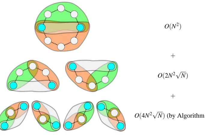
The marginalization steps of Algorithm 5 (lines 2, 3, and 4) may further decompose into smaller groups, in which case Algorithm 5 can be applied recursively. For instance, the graph in Figure 7(a) represents the marginalization step that is to be performed in Figure 6(c) (Algorithm 5, line 4). Since this marginalization step is the asymptotically dominant step in the algorithm, applying Algorithm 5 recursively lowers the asymptotic complexity.

Another straightforward example of applying recursion in Algorithm 5 is shown in Figure 8, in which a ring-structured model is marginalized with respect to two of its nodes. Doing so takes

(16)

Description lines time

Marginalization ofΦX, without recursion 2 Θ(N|X|)

Marginalization ofΦY 3 Θ(N|Y|)

Marginalization ofΦZ 4 Θ(N|Z|)

SortingΦY 5–7 Θ(|Y′\X|N|Y

′_| log N)

SortingΦZ 8–10 Θ(|Z′\X|N|Z

′_| log N)

Running Algorithm 2 on the sorted values 11–16 O(N|X′|√N|(Y′_∩_Z′₎_\_X′_|₎

Table 2: Detailed running time analysis of Algorithm 5; any of these terms may be asymptotically dominant

Graph:

{A complete graph KM,

with pairwise terms}

(a) (b) (c) (d) (e)

Algorithm 1: Θ(N5) Θ(N3) Θ(N11) Θ(N6) Θ(NM)

Algorithm 5: O(N3√N) O(N2√N) O(N6√N) O(N5) O(N5M/6)

Speed-up: Ω(N√N) Ω(√N) Ω(N4√N) Ω(N) Ω(NM/6)

Figure 7: Some example graphs whose max-marginals are to be computed with respect to the col-ored nodes, using the three regions shown. Factors are indicated using differently colcol-ored edges, while dotted edges always indicate pairwise factors. (a) is the region Z from Fig-ure 6 (recursion is applied again to achieve this result); (b) is the graph used to motivate Algorithm 4; (c) shows a query in a graph with regular structure; (d) shows a complete graph with six nodes; (e) generalizes this to a clique with M nodes.

that our algorithm will be faster if the number of iterations isΩ(√N). Naturally, Algorithm 4 could be applied directly to the triangulated graph, which would again take O(MN2√N).

5.3 A General Extension to Higher-Order Cliques

Naturally, there are cases for which a decomposition into three terms is not possible, such as

mi,j,k(xi,xj,xk) =max xm

Φi,j,k(xi,xj,xk)×Φi,j,m(xi,xj,xm)×

Φi,k,m(xi,xk,xm)×Φj,k,m(xj,xk,xm) (13)

(i.e., a clique of size four with all possible third-order factors). However, if the model contains factors of size K, it must always be possible to split it into K+1 groups (e.g., four in the case of Equation 13).

Our optimizations can easily be applied in these cases simply by adapting Algorithm 2 to solve problems of the form

max

(17)

O(N2₎

+

O(2N2√N)

+

O(4N2√N)(by Algorithm 4)

Figure 8: In the above example, lines 2–4 of Algorithm 5 are applied recursively, achieving a total running time of O(MN2√N)for a loop with M nodes (our algorithm achieves the same running time in the triangulated graph).

Step 1:                

              

6 2 14 16 9 7 12 8 10 3 11 13 1 15 4 5 99 92 87 81 78 66 53 46 30 26 21 16 12 10 8 6

3 4 8 11 7 16 13 9 6 2 15 10 12 5 1 14 98 93 85 76 71 70 67 65 63 57 48 42 39 37 26 17

don't search past this line

11 4 5 10 14 6 9 7 3 16 12 2 8 13 15 1 97 95 81 78 75 60 55 50 44 39 37 31 30 27 26 20

Figure 9: Algorithm 2 can easily be extended to cases including more than two sequences.

Pseudocode for this extension is presented in Algorithm 6. Note carefully the use of the variable

read: we are storing which indices have been read to avoid re-reading them; this guarantees that

our Algorithm is never asymptotically worse than the na¨ıve solution. Figure 9 demonstrates how such an algorithm behaves in practice. Again, we shall discuss the running time of this extension in Appendix A. For the moment, we state the following theorem:

Theorem 3 Algorithm 6 generalizes Algorithm 2 to K lists with an expected running time of O(KNKK−1),

yielding a speed-up of at leastΩ(1 KN

1

K)in cliques containing K-ary factors. It is never worse than

the na¨ıve solution, meaning that it takes O(min(N,KNK−K1)).

(18)

Algorithm 6 Find i such that∏K_k₌₁vk[i]is maximized

Input: K vectors v1. . .vK; permutation functions p1. . .pK that sort them in decreasing order; a

vector read indicating which indices have been read, and a unique value T _∈/read _{read is

essentially a boolean array indicating which indices have been read; since creating this array is an O(N)operation, we create it externally, and reuse it O(N)times; setting read[i] =T indicates

that a particular index has been read; we use a different value of T for each call to this function so that read can be reused without having to be reinitialized_}

1: Initialize: start :=1,

max :=maxp∈{p1...pK}∏

K

k=1vk[p[1]], best :=argmax_p_∈{_p₁_..._p_K_}∏K_k₌₁vk[p[1]] 2: for k_{∈ {}1. . .K_}do

3: endk:=maxq∈{p1...pK}p

−1

k [q[1]] 4: read[pk[1]] =T

5: end for

6: while start<max{end1. . .endK}do 7: start :=start+1

8: for k_{∈ {}1. . .K_}do

9: if read[pk[start]]:=T then 10: continue

11: end if

12: read[pk[start]]:=T 13: m :=∏K_x₌₁vx[pk[start]] 14: if m>max then 15: best :=pk[start] 16: max :=m 17: end if

18: ek:=maxq∈{p1...pK}p−

1

k [q[start]] 19: endk:=min(ek,endk)

20: end for

21: end while_{see Appendix A for running times_}

22: Return: best

about K groups _{G1. . .GK}, and calls to Algorithm 2 become calls to Algorithm 6). The one

remaining case that has not been considered is when the sequences v1···vKare functions of different

(but overlapping) variables; na¨ıvely, we can create a new variable whose domain is the product space of all of the overlapping terms, and still achieve the performance improvement guaranteed by Theorem 3; in some cases, better results can again be obtained by applying recursion, as in Figure 7.

As a final comment we note that we have not provided an algorithm for choosing how to split the variables of a model into(K+1)-groups. We note even if we split the groups in a na¨ıve way, we are guaranteed to get at least the performance improvement guaranteed by Theorem 3, though more ‘intelligent’ splits may further improve the performance.

(19)

5.4 Extensions for Conditionally Factorizable Models

Just as in Section 5.2, we can extend Algorithm 3 to factors of any size, so long as the purely latent cliques contain more latent variables than those cliques that depend upon the observation. The analysis for this type of model is almost exactly the same as that presented in Section 5.2, except that any terms consisting of purely latent variables are processed offline.

As we mentioned in 5.2, if a model contains (non-maximal) factors of size K, we will gain a speed-up ofΩ(_K1NK1). If in addition there is a factor (either maximal or non-maximal) consisting

of purely latent variables, we can still obtain a speed-up ofΩ( 1 K+1N

1

K+1)_{, since this factor merely}

contributes an additional term to (Equation 14). Thus when our ‘data-dependent’ terms contain only a single latent variable (i.e., K=1), we gain a speed-up ofΩ(√N), as in Algorithm 3.

6. Performance Improvements in Existing Applications

Our results are immediately compatible with several applications that rely on inference in graphical models. As we have mentioned, our results apply to any model whose cliques decompose into

lower-order terms.

Often, potentials are defined only on nodes and edges of a model. A Dth-order Markov model has a tree-width of D, despite often containing only pairwise relationships. Similarly ‘skip-chain CRFs’ (Sutton and McCallum, 2006; Galley, 2006), and junction-trees used in SLAM applications (Paskin, 2003) often contain only pairwise terms, and may have low tree-width under reasonable conditions. These are examples of latently factorizable models. In each case, if the tree-width is

D, Algorithm 5 takes O(MND√N)(for a model with M nodes and N states per node), yielding a speed-up ofΩ(√N).

Models for shape-matching and pose reconstruction often exhibit similar properties (Tresadern et al., 2009; Donner et al., 2007; Sigal and Black, 2006). In each case, third-order cliques factorize into second-order terms; hence we can apply Algorithm 4 to achieve a speed-up ofΩ(√N).

Another similar model for shape-matching is that of Felzenszwalb (2005); this model again contains third-order cliques, though it includes a ‘geometric’ term constraining all three variables. Here, the third-order term is independent of the input data, meaning that each of its rows can be sorted offline, as described in Section 3. This is an example of a conditionally factorizable model. In this case, those factors that depend upon the observation are pairwise, meaning that we achieve a speed-up ofΩ(N13). Further applications of this type shall be explored in Section 7.4.

In Coughlan and Ferreira (2002), deformable shape-matching is solved approximately using loopy belief-propagation. Their model has only second-order cliques, meaning that inference takes

Θ(MN2)per iteration. Although we cannot improve upon this result, we note that we can typically

do exact inference in a single iteration in O(MN2√N); thus our model has the same running time as

O(√N)iterations of the original version. This result applies to all second-order models containing a single loop (Weiss, 2000).

In McAuley et al. (2008), a model is presented for graph-matching using loopy belief-propagation; the maximal cliques for D-dimensional matching have size(D+1), meaning that inference takes

Θ(MND+1) per iteration (it is shown to converge to the correct solution); we improve this to O(MND√N).

Interval graphs can be used to model resource allocation problems (Fulkerson and Gross, 1965);

(20)

Reference description running time our method McAuley et al. (2008) D-d graph-matching Θ(MND+1)(iter.) O(MND√N)(iter.)

Sutton and McCallum (2006) Width-D skip-chain O(MND) O(MND−1√N)

Galley (2006) Width-3 skip-chain Θ(MN3) O(MN2√N)

Tresadern et al. (2009) Deformable matching Θ(MN3) O(MN2√N)

Coughlan and Ferreira (2002) Deformable matching Θ(MN2)(iter.) O(MN2√N)

Sigal and Black (2006) Pose reconstruction Θ(MN3) O(MN2√N)

Felzenszwalb (2005) Deformable matching Θ(MN3) Θ(MN83)(online)

Fulkerson and Gross (1965) Width-D interval graph O(MND+1) O(MND√N)

Table 3: Some existing work to which our results can be immediately applied (M is the number of nodes in the model, N is the number of states per node. ‘iter.’ denotes that the algorithm is iterative).

number of overlapping requests, though the constraints are only pairwise, meaning that we again achieve anΩ(√N)improvement.

Finally, in Section 7.4 we shall explore a variety of applications in which we have pairwise models of the form shown in (Equation 7). In all of these cases, we see an (expected) reduction of aΘ(MN2)message-passing algorithm to O(MN√N).

Table 3 summarizes these results. Reported running times reflect the expected case. Note that we are assuming that max-product belief-propagation is being used in a discrete model; some of the referenced articles may use different variants of the algorithm (e.g., Gaussian models, or approxi-mate inference schemes). We believe that our improvements may revive the exact, discrete version as a tractable option in these cases.

7. Experiments

We present experimental results for two types of models: latently factorizable models, whose cliques factorize into smaller terms, as discussed in Section 4, and conditionally factorizable models, whose factors that depend upon the observation contain fewer latent variables than their maximal cliques, as discussed in Section 3.

We begin with an asymptotic analysis of the running time of our algorithm on the ‘inner product’ operations of (Equation 1) and (Equation 14), in order to assess Theorems 2 and 3 experimentally.

7.1 Comparison Between Asymptotic Performance and Upper-Bounds

For our first experiment, we compare the performance of Algorithms 2 and 6 to the na¨ıve solution of Algorithm 1. These are core subroutines of each of the other algorithms, meaning that determining their performance shall give us an accurate indication of the improvements we expect to obtain in real graphical models.

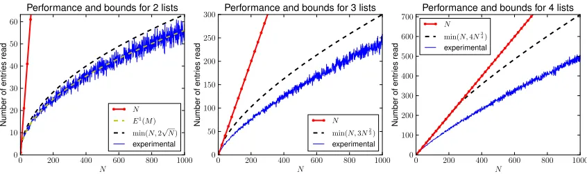
For each experiment, we generate N i.i.d. samples from [0,1)to obtain the lists v1. . .vK. N is

(21)

0 200 400 600 800 1000 N 0 10 20 30 40 50 60 Number of entr ies read

Performance and bounds for 2 lists

N E1

(M) min(N,2√N) experimental

N

min(N,3N23₎

experimental

0 200 400 600 800 1000 N 0 100 200 300 400 500 600 700 Number of entr ies read

N

min(N,4N3 4)

experimental

Figure 10: Performance of our algorithm and bounds. For K=2, the exact expectation is shown, which appears to precisely match the average performance (over 100 trials). The dotted lines show the bound of (Equation 23). While the bound is close to the true performance for K=2, it becomes increasingly loose for larger K.

of size 5); therefore smaller values of K are probably more realistic in practice (indeed, all of the applications in Section 6 have K=2).

The performance of our algorithm is shown in Figure 10, for K =2 to 4 (i.e., for 2 to 4 lists). When K=2, we execute Algorithm 2, while Algorithm 6 is executed for K_≥3. The performance reported is simply the number of elements read from the lists (which is at most K_×start). This

is compared to N itself, which is the number of elements read by the na¨ıve algorithm. The upper-bounds we obtained in (Equation 23) are also reported, while the true expected performance (i.e., Equation 19) is reported for K=2. Note that the variable read was introduced into Algorithm 6 in order to guarantee that it can never be asymptotically slower than the na¨ıve algorithm. If this variable is ignored, the performance of our algorithm deteriorates to the point that it closely approaches the upper-bounds shown in Figure 10. Unfortunately, this optimization proved overly complicated to include in our analysis, meaning that our upper-bounds remain highly conservative for large K.

7.2 Performance Improvement for Dependent Variables

The expected-case running time of our algorithm was derived under the assumption that each list has independent order statistics, as was the case for our previous experiment. We suggested that we will obtain worse performance in the case of negatively correlated variables, and better performance in the case of positively correlated variables; we shall assess these claims in this experiment.

Figure 11 shows how the order statistics of va and vbcan affect the performance of our

algo-rithm. Essentially, the running time of Algorithm 2 is determined by the level of ‘diagonalness’ of the permutation matrices in Figure 11; highly diagonal matrices result in better performance than the expected case, while highly off-diagonal matrices result in worse performance. The expected case was simply obtained under the assumption that every permutation is equally likely.

We report the performance for two lists (i.e., for Algorithm 2), where each (va[i],vb[i])is an

independent sample from a 2-dimensional Gaussian with covariance matrix

(22)

←best case

permutation:

operations: 1 1 3 3 5

worst case_→

permutation

operations: 7 7 9 10 10

Figure 11: Different permutation matrices and their resulting cost (in terms of entries read/multiplications performed). Each permutation matrix transforms the sorted val-ues of one list into the sorted valval-ues of the other, that is, it transforms vaas sorted by pa

into vbas sorted by pb. The red (lighter) squares show the entries that must be read

be-fore the algorithm terminates (each corresponding to one multiplication). See Figure 23 for further explanation.

meaning that the two lists are correlated with correlation coefficient c (here we are working in the max-sum semiring). This dependence between the values of the two lists leads to a dependence in their order statistics, so that in the case of Gaussian random variables, the correlation coefficient precisely captures the ‘diagonalness’ of the matrices in Figure 11. Performance is shown in Fig-ure 12 for different values of c (c=0, is not shown, as this is the case observed in the previous experiment).

7.3 Message-Passing in Latently Factorizable Models

In this section we present experiments in models whose cliques factorize into smaller terms, as discussed in Section 4.

7.3.1 2-DIMENSIONALGRAPH-MATCHING

Naturally, Algorithm 5 has additional overhead compared to the na¨ıve solution, meaning that it will not be beneficial for small N. In this experiment, we aim to assess the extent to which our approach is faster in real applications. We reproduce the model from McAuley et al. (2008), which performs 2-dimensional graph-matching, using a loopy graph with cliques of size three, containing only second-order potentials (as described in Section 6); the Θ(NM3) performance of McAuley et al. (2008) is reportedly state-of-the-art. We also show the performance on a graphical model with

random potentials, in order to assess how the results of the previous experiments are reflected in

(23)

Performance and bounds forc_{= 0}.₂

N E1

Performance and bounds forc_{= 0}.₅

N E1

Performance and bounds forc_{= 1}.₀

N E1

0 200 400 600 800 1000 N 0 20 40 60 80 100 Number of entr ies read

Performance and bounds forc₌₋₀.₂

N E1₍_M₎ min(N,2√N) experimental

0 200 400 600 800 1000 N 0 50 100 150 200 Number of entr ies read

Performance and bounds forc₌₋₀.₅

N E1₍_M₎ min(N,2√N) experimental

0 200 400 600 800 1000 N 0 200 400 600 800 1000 Number of entr ies read

Performance and bounds forc₌₋₁.₀

N E1

Figure 12: Performance of our algorithm for different correlation coefficients. The top three plots show positive correlation, the bottom three show negative correlation. Correlation coef-ficients of c=1.0 and c=₋1.0 capture precisely the best and worst-case performance of our algorithm, resulting in O(1)andΘ(N)performance, respectively (when c=₋1.0 the linear curve obscures the experimental curve).

We perform matching between a template graph with M nodes, and a target graph with N nodes, which requires a graphical model with M nodes and N states per node (see McAuley et al. 2008 for details). We fix M=10 and vary N.

Figure 13 (left) shows the performance on random potentials, that is, the performance we hope to obtain if our model assumptions are satisfied. Figure 13 (right) shows the performance for graph-matching, which closely matches the expected-case behavior. Fitted curves are shown together with the actual running time of our algorithm, confirming its O(MN2√N)performance. The coefficients of the fitted curves demonstrate that our algorithm is useful even for modest values of N.

We also report results for graph-matching using graphs from the MPEG-7 data set (Bai et al., 2009), which consists of 1,400 silhouette images (Figure 14). Again we fix M=10 (i.e., 10 points are extracted in each template graph) and vary N (the number of points in the target graph). This experiment confirms that even when matching real-world graphs, the assumption of independent order statistics appears to be reasonable.

7.3.2 HIGHER-ORDERMARKOVMODELS

(24)

0 100 200 300 400 500 600 700 800 N(number of states)

0 50 100 150 200 250 300 350 400 450

A

ver

age

w

all

time

(seconds)

Random potentials (5 iterations)

na¨ıve method 0._00000079N3

(r_{= 546}.₃₃₎ our method

0._00000388N2.5(r= 30.06)

0 100 200 300 400 500 600 700 800 N(size of target graph)

0 100 200 300 400 500

A

ver

age

w

all

time

(seconds)

2D Graph matching

(r_{= 361}.₆₁₎ our method

0._00000422N2.5(r= 11.60)

Figure 13: The running time of our method on randomly generated potentials, and on a graph-matching experiment (both graphs have the same topology). Fitted curves are also ob-tained by performing least-squares regression; the residual error r indicates the ‘good-ness’ of the fitted curve.

0 100 200 300 400 500 N(size of target graph)

0 5 10 15 20 25 30 35

A

ver

age

w

all

time

(seconds)

2D Graph matching (MPEG-7 data)

(r_{= 14}.₇₃₅₅₆₎ our method

0._00000095N2.5(r= 0.01651)

Figure 14: The running time of method our on graphs from the MPEG-7 data set.

wondrous sight of th4 ivory Pequod is corrected to wondrous sight of the ivory Pequod.

(25)

Figure 15: Left: Our model for denoising. Its computational complexity is similar to that of a skip-chain CRF, and models for named-entity recognition (right).

Specifically, our model takes the form

ΦX(xX) =

|X|−1

∏

i=1

Φi,i+1(xi,xi+1)×

|X|−2

∏

i=1

Φi,i+2(xi,xi+2)

where

Φi,j(xi,xj) =ψi,j(xi,xj)p(xi|oi)p(xj|oj).

Hereψis our prior (extracted from text statistics), and p is our ‘noise model’ (given the observation

o). The computational complexity of inference in this model is similar to that of the skip-chain CRF

shown in Figure 3(b), as well as models for part-of-speech tagging and named-entity recognition, as in Figure 15. Text denoising is useful for the purpose of demonstrating our algorithm, as there are several different corpora available in different languages, allowing us to explore the effect that the domain size (i.e., the size of the language’s alphabet) has on running time.

We extracted pairwise statistics based on 10,000 characters of text, and used this to correct a series of 25 character sequences, with 1% random noise introduced to the text. The domain was simply the set of characters observed in each corpus. The Japanese data set was not included, as the

Θ(MN2)memory requirements of the algorithm made it infeasible with N_≃2000; this is addressed in Section 7.4.1.

The running time of our method, compared to the na¨ıve solution, is shown in Figure 16. One might expect that texts from different languages would exhibit different dependence structures in their order statistics, and therefore deviate from the expected case in some instances. However, the running times appear to follow the fitted curve closely, that is, we are achieving approximately the expected-case performance in all cases.

Since the priorψi,i+1(xi,xi+1)is data-independent, we shall further discuss this type of model

in reference to Algorithm 3 in Section 7.4.

7.4 Experiments with Conditionally Factorizable Models

In each of the following experiments we perform belief-propagation in models of the form given in (Equation 7). Thus each model is completely specified by defining the node potentialsΦi(xi|yi), the

edge potentialsΦi,j(xi,xj), and the topology(N,

E

)of the graph.

Furthermore we assume that the edge potentials are homogeneous, that is, that the potential for each edge is the same, or rather that they have the same order statistics (for example, they may differ by a multiplicative constant). This means that sorting can be done online without affecting the asymptotic complexity. When subject to heterogeneous potentials we need merely sort them