Practical Kernel-Based Reinforcement Learning
Andr´e M. S. Barreto [email protected]
Laborat´orio Nacional de Computa¸c˜ao Cient´ıfica Petr´opolis, Brazil
Doina Precup [email protected]
Joelle Pineau [email protected]
School of Computer Science McGill University
Montreal, Canada
Editor:George Konidaris
Abstract
Kernel-based reinforcement learning(KBRL) stands out among approximate reinforcement learning algorithms for its strong theoretical guarantees. By casting the learning problem as a local kernel approximation, KBRL provides a way of computing a decision policy which converges to a unique solution and is statistically consistent. Unfortunately, the model constructed by KBRL grows with the number of sample transitions, resulting in a computational cost that precludes its application to large-scale or on-line domains. In this paper we introduce an algorithm that turns KBRL into a practical reinforcement learn-ing tool. Kernel-based stochastic factorization (KBSF) builds on a simple idea: when a transition probability matrix is represented as the product of two stochastic matrices, one can swap the factors of the multiplication to obtain another transition matrix, potentially much smaller than the original, which retains some fundamental properties of its precursor. KBSF exploits such an insight to compress the information contained in KBRL’s model into an approximator of fixed size. This makes it possible to build an approximation con-sidering both the difficulty of the problem and the associated computational cost. KBSF’s computational complexity is linear in the number of sample transitions, which is the best one can do without discarding data. Moreover, the algorithm’s simple mechanics allow for a fully incremental implementation that makes the amount of memory used independent of the number of sample transitions. The result is a kernel-based reinforcement learning algorithm that can be applied to large-scale problems in both off-line and on-line regimes. We derive upper bounds for the distance between the value functions computed by KBRL and KBSF using the same data. We also prove that it is possible to control the magnitude of the variables appearing in our bounds, which means that, given enough computational resources, we can make KBSF’s value function as close as desired to the value function that would be computed by KBRL using the same set of sample transitions. The potential of our algorithm is demonstrated in an extensive empirical study in which KBSF is ap-plied to difficult tasks based on real-world data. Not only does KBSF solve problems that had never been solved before, but it also significantly outperforms other state-of-the-art reinforcement learning algorithms on the tasks studied.
long-sought goal in artificial intelligence: the construction of situated agents that learn how to behave from direct interaction with the environment (Sutton and Barto, 1998). But such an endeavor does not come without its challenges; among them, extrapolating the field’s basic machinery to large-scale domains has been a particularly persistent obstacle.
It has long been recognized that virtually any real-world application of reinforcement learning must involve some form of approximation. Given the mature stage of the supervised-learning theory, and considering the multitude of approximation techniques available today, this realization may not come across as a particularly worrisome issue at first glance. How-ever, it is well known that the sequential nature of the reinforcement learning problem renders the incorporation of function approximators non-trivial (Bertsekas and Tsitsiklis, 1996).
Despite the difficulties, in the last two decades the collective effort of the reinforcement learning community has given rise to many reliable approximate algorithms (Szepesv´ari, 2010). Among them, Ormoneit and Sen’s (2002) kernel-based reinforcement learning (KBRL) stands out for two reasons. First, unlike other approximation schemes, KBRL always con-verges to a unique solution. Second, KBRL is consistent in the statistical sense, meaning that adding more data improves the quality of the resulting policy and eventually leads to optimal performance.
Unfortunately, the good theoretical properties of KBRL come at a price: since the model constructed by this algorithm grows with the number of sample transitions, the cost of computing a decision policy quickly becomes prohibitive as more data become available. Such a computational burden severely limits the applicability of KBRL. This may help explain why, in spite of its nice theoretical guarantees, kernel-based learning has not been widely adopted as a practical reinforcement learning tool.
This paper presents an algorithm that can potentially change this situation. Kernel-based stochastic factorization(KBSF) builds on a simple idea: when a transition probability matrix is represented as the product of two stochastic matrices, one can swap the factors of the multiplication to obtain another transition matrix, potentially much smaller than the original, which retains some fundamental properties of its precursor (Barreto and Fragoso, 2011). KBSF exploits this insight to compress the information contained in KBRL’s model into an approximator of fixed size. Specifically, KBSF builds a model, whose size is inde-pendent of the number of sample transitions, which serves as an approximation of the model that would be constructed by KBRL. Since the size of the model becomes a parameter of the algorithm, KBSF essentially detaches the structure of KBRL’s approximator from its configuration. This extra flexibility makes it possible to build an approximation that takes into account both the difficulty of the problem and the computational cost of finding a policy using the constructed model.
we present an extensive empirical study in which KBSF is applied to difficult control tasks based on real-world data, some of which had never been solved before. KBSF outperforms least-squares policy iteration and fittedQ-iteration on several off-line problems and SARSA on a difficult on-line task.
We also show that KBSF is a sound algorithm from a theoretical point of view. Specifi-cally, we derive results bounding the distance between the value function computed by our algorithm and the one computed by KBRL using the same data. We also prove that it is possible to control the magnitude of the variables appearing in our bounds, which means that we can make the difference between KBSF’s and KBRL’s solutions arbitrarily small.
We start the paper presenting some background material in Section 2. Then, in Sec-tion 3, we introduce the stochastic-factorizaSec-tion trick, the insight underlying the devel-opment of our algorithm. KBSF itself is presented in Section 4. This section is divided in two parts, one theoretical and one practical. In Section 4.1 we present theoretical re-sults showing that not only is the difference between KBSF’s and KBRL’s value functions bounded, but it can also be controlled. Section 4.2 brings experiments with KBSF on four reinforcement-learning problems: single and double pole-balancing, HIV drug schedule do-main, and epilepsy suppression task. In Section 5 we introduce the incremental version of our algorithm, which can be applied to on-line problems. This section follows the same structure of Section 4, with theoretical results followed by experiments. Specifically, in Sec-tion 5.1 we extend the results of SecSec-tion 4.1 to the on-line scenario, and in SecSec-tion 5.2 we present experiments on the triple pole-balancing and helicopter tasks. In Section 6 we take a closer look at the approximation computed by KBSF and present a practical guide on how to configure our algorithm to solve a reinforcement learning problem. In Section 7 we sum-marize related works and situate KBSF in the context of kernel-based learning. Finally, in Section 8 we present the main conclusions regarding the current research and discuss some possibilities of future work.
The paper has three appendices. Appendix A has the proofs of our theoretical results. The details of the experiments that were omitted in the main body of the text are described in Appendix B. In Appendix C we provide a table with the main symbols used in the paper that can be used as a reference to facilitate reading.
Parts of the material presented in this article have appeared before in two papers pub-lished in theNeural Information Processing Systemsconference (NIPS, Barreto et al., 2011, 2012). The current manuscript is a substantial extension of the aforementioned works.
2. Background
We consider the standard framework of reinforcement learning, in which anagent interacts with an environment and tries to maximize the amount of reward collected in the long run (Sutton and Barto, 1998). The interaction between agent and environment happens at discrete time steps: at each instant t the agent occupies a states(t) ∈S and must choose an action a from a finite set A. The sets S and A are called the state and action spaces, respectively. The execution of action ain state s(t) moves the agent to a new states(t+1), where a new action must be selected, and so on. Each transition has a certain probability of occurrence and is associated with a reward r ∈ R. The goal of the agent is to find a
R(t)=r(t+1)+γr(t+2)+γ2r(t+3)+...=
i=1
γi−1r(t+i), (1)
where r(t+1) is the reward received at the transition from state s(t) to state s(t+1). The interaction of the agent with the environment may last forever (T =∞) or until the agent reaches a terminal state (T < ∞); each sequence of interactions is usually referred to as an episode. The parameter γ ∈[0,1) is the discount factor, which determines the relative importance of individual rewards depending on how far in the future they are received.
2.1 Markov Decision Processes
As usual, we assume that the interaction between agent and environment can be mod-eled as a Markov decision process (MDP, Puterman, 1994). An MDP is a tuple M ≡ (S, A, Pa, Ra, γ), where Pa and Ra describe the dynamics of the task at hand. For each action a ∈ A, Pa(·|s) defines the next-state distribution upon taking action a in state s. The reward received at transitions−→a s0 is given byRa(s, s0), with|Ra(s, s0)| ≤R
max<∞. Usually, one is interested in the expected reward resulting from the execution of action a
in states, that is,ra(s) =Es0∼Pa(·|s){Ra(s, s0)}.
Once the interaction between agent and environment has been modeled as an MDP, a natural way of searching for an optimal policy is to resort to dynamic programming (Bell-man, 1957). Central to the theory of dynamic-programming is the concept of a value function. The value of state s under a policy π, denoted by Vπ(s), is the expected re-turn the agent will receive from s when following π, that is, Vπ(s) = Eπ{R(t)|s(t) = s} (here the expectation is over all possible sequences of rewards in (1) when the agent fol-lows π). Similarly, the value of the state-action pair (s, a) under policy π is defined as
Qπ(s, a) =E
s0∼Pa(·|s){Ra(s, s0) +γVπ(s0)}=ra(s) +γEs0∼Pa(·|s){Vπ(s0)}.
The notion of value function makes it possible to impose a partial ordering over decision policies. In particular, a policy π0 is considered to be at least as good as another policy π
if Vπ0(s) ≥ Vπ(s) for all s ∈ S. The goal of dynamic programming is to find an optimal policyπ∗ that performs no worse than any other. It is well known that there always exists at least one such policy for a given MDP (Puterman, 1994). When there is more than one optimal policy, they all share the same value functionV∗.
When both the state and action spaces are finite, an MDP can be represented in matrix form: each function Pa becomes a matrix Pa ∈ R|S|×|S|, with pa
ij = Pa(sj|si), and each
functionrabecomes a vectorra ∈R|S|, wherera
i =ra(si). Similarly,Vπ can be represented
as a vector vπ ∈R|S| and Qπ can be seen as a matrixQπ ∈R|S|×|A|. 1
When the MDP is finite, dynamic programming can be used to find an optimal decision-policyπ∗ ∈A|S| in time polynomial in the number of states|S|and actions|A|(Ye, 2011).
Letv∈R|S|and letQ∈
R|S|×|A|. Define the operator Γ :R|S|×|A|7→R|S|such that ΓQ=v
if and only ifvi = maxjqij for alli. Also, given an MDPM, define ∆ :R|S|7→R|S|×|A|such
that ∆v=Qif and only ifqia=rai +γP|S|
j=1paijvj for all iand alla. TheBellman operator
of the MDPM is given by T ≡Γ∆. A fundamental result in dynamic programming states that, starting fromv(0)=0, the expressionv(t)=Tv(t−1)= ΓQ(t)gives the optimalt-step value function, and as t → ∞ the vector v(t) approaches v∗. At any point, the optimal
t-step policy can be obtained by selectingπi(t) ∈argmaxjq(ijt) (Puterman, 1994).
In contrast with dynamic programming, in reinforcement learning it is assumed that the MDP is unknown, and the agent must learn a policy based on transitions sampled from the environment. If the process of learning a decision policy is based on a fixed set of sample transitions, we call it batch reinforcement learning. On the other hand, in on-line reinforcement learning the computation of a decision policy takes place concomitantly with the collection of data (Sutton and Barto, 1998).
2.2 Kernel-Based Reinforcement Learning
Kernel-based reinforcement learning (KBRL) is a batch algorithm that uses a finite model approximation to solve a continuous MDPM ≡(S, A, Pa, Ra, γ), whereS⊆[0,1]dSandd
S∈
N+∗ is the dimension of the state space (Ormoneit and Sen, 2002). LetSa≡ {(sak, rka,sˆak)|k=
1,2, ..., na}be sample transitions associated with actiona∈A, wheresak,ˆsak ∈Sandrak∈R.
Letφ:R+7→R+ be a Lipschitz continuous function satisfyingR01φ(x)dx= 1. Let kτ(s, s0)
be a kernel function defined as
kτ(s, s0) =φ
ks−s0k τ
, (2)
where τ ∈R and k · k is a norm in RdS (for concreteness, the reader may think of kτ(s, s0)
as the Gaussian kernel, although the definition also encompasses other functions). Finally, define the normalized kernel function associated with action aas
κaτ(s, sai) = kτ(s, s
a i)
Pna
j=1kτ(s, saj)
. (3)
KBRL uses (3) to build a finite MDP whose state space ˆS is composed solely of the n=
P
anastates ˆsai. We assume without loss of generality that the action spaceAis ordered and
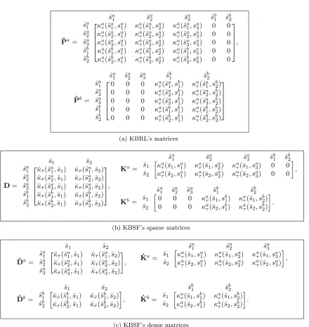
the sampled states are ordered lexicographically as ˆsai <sˆbj ⇐⇒ a < b or (a=band i < j); if a given states∈Soccurs more than once in the set of sample transitions, each occurrence will be treated as a distinct state in the finite MDP. The transition functions of KBRL’s model, ˆPa: ˆS×Sˆ7→[0,1], are given by:
ˆ
Paˆsbi|s=
κaτ(s, sbi), ifa=b,
0, otherwise, (4)
where a, b ∈ A. Similarly, the reward functions of the MDP constructed by KBRL, ˆRa : ˆ
S×Sˆ7→R, are
ˆ
Ra(s,sˆbi) =
ria, ifa=b,
replacing s with the sampled states ˆsi (see Figure 2a). The vectorsˆr are computed as follows. Let r≡ [(r1)|,(r2)|, ...,(r|A|)|]| ∈Rn, where ra ∈
Rna are the vectors composed
of the sample rewards, that is, the ith element of ra is rai ∈ Sa. Since Ra(s,sˆbi) does not depend on the start states, we can write
ˆra=Pˆar. (6)
KBRL’s MDP is thus given by ˆM ≡( ˆS, A,Pˆa,ˆra, γ).
Once ˆM has been defined, one can use dynamic programming to compute its optimal value function ˆV∗. Then, the value of any state-action pair of the continuous MDP can be determined as:
ˆ
Q(s, a) =
na
X
i=1
κaτ(s, sai)
h
ria+γVˆ∗(ˆsai)
i
, (7)
where s ∈ S and a ∈ A. Ormoneit and Sen (2002) have shown that, if na → ∞ for all a∈A and the kernel’s width τ shrink at an “admissible” rate, the probability of choosing a suboptimal action based on ˆQ(s, a) converges to zero (see their Theorem 4).
As discussed, using dynamic programming one can compute the optimal value function of ˆM in time polynomial in the number of sample transitionsn(which is also the number of states in ˆM). However, since each application of the Bellman operator ˆT is O(n2|A|), the computational cost of such a procedure can easily become prohibitive in practice. Thus, the use of KBRL leads to a dilemma: on the one hand one wants as much data as possible to describe the dynamics of the task, but on the other hand the number of transitions should be small enough to allow for the numerical solution of the resulting model. In the following sections we describe a practical approach to weigh the relative importance of these two conflicting objectives.
3. Stochastic Factorization
A stochastic matrix has only nonnegative elements and each of its rows sums to 1. That said, we can introduce the concept that will serve as a cornerstone for the rest of the paper:
Definition 1 Given a stochastic matrix P ∈ Rn×p, the relation P = DK is called a
stochastic factorization of P if D ∈ Rn×m and K ∈
Rm×p are also stochastic matrices.
The integer m >0 is the order of the factorization.
This mathematical construct has been explored before. For example, Cohen and Roth-blum (1991) briefly discuss it as a special case of nonnegative matrix factorization, while Cut-ler and Breiman (1994) study slightly modified versions of stochastic factorization for sta-tistical data analysis. However, in this paper we will focus on a useful property of this type of factorization that has only recently been noted (Barreto and Fragoso, 2011).
P=
× × 0 × × × × 0 ×
D=
× 0 × × 0 ×
K=
× × 0 × 0 ×
¯ P=
× × × ×
Figure 1: Reducing the dimension of a transition model fromn= 3 states tom= 2 artificial states. Original statessi are represented as big white circles; small black circles
depict artificial states ¯sh. The symbol ‘×’ is used to represent nonzero elements.
These figures have appeared before in the article by Barreto and Fragoso (2011).
D and K as probabilities of transitions between the states si and a set of m artificial
states ¯sh. Specifically, the elements in each row of D can be interpreted as probabilities
of transitions from the original states to the artificial states, while the rows of K can be seen as probabilities of transitions in the opposite direction. Under this interpretation, each element pij =Pmh=1dihkhj is the sum of the probabilities associated with m two-step
transitions: from statesito each artificial state ¯sh and from these back to statesj. In other words,pij is the accumulated probability of all possible paths fromsi tosj with a stopover in one of the artificial states ¯sh. Following similar reasoning, it is not difficult to see that by
swapping the factors of a stochastic factorization, that is, by switching from DK toKD, one obtains the transition probabilities between the artificial states ¯sh,P¯ =KD. Ifm < n,
¯
P ∈ Rm×m will be a compact version of P. Figure 1 illustrates this idea for the case in
which n= 3 and m= 2.
The stochasticity ofP¯ follows immediately from the same property ofDandK. What is perhaps more surprising is the fact that this matrix shares some fundamental characteristics with the original matrix P. Specifically, it is possible to show that: (i) for each recurrent class inPthere is a corresponding class inP¯ with the same period and, given some simple assumptions about the factorization, (ii) Pis irreducible if and only ifP¯ is irreducible and (iii) P is regular if and only if P¯ is regular (for details, see the article by Barreto and Fragoso, 2011). We will refer to this insight as the “stochastic-factorization trick”:
Given a stochastic factorization of a transition matrix, P= DK, swapping the factors of the factorization yields another transition matrix P¯ =KD, potentially much smaller than the original, which retains the basic topology and properties ofP.
Given the strong connection between P∈ Rn×n and P¯ ∈
Rm×m, the idea of replacing
stochastic-factorization trick to reduce the computational cost of KBRL. The strategy will be to summarize the information contained in KBRL’s MDP in a model of fixed size.
3.2 Reducing a Markov Decision Process
The idea of using stochastic factorization to reduce dynamic programming’s computational requirements is straightforward: given factorizations of the transition matrices Pa, we can
apply our trick to obtain a reduced MDP that will be solved in place of the original one. In the most general scenario, we would have one independent factorizationPa=DaKafor each action a∈A and then use P¯a=KaDa instead of Pa. However, in the current work
we will focus on the particular case in which there is a single matrixD, which will prove to be convenient both mathematically and computationally.
Obviously, in order to apply the stochastic-factorization trick to an MDP, we have to first compute the matrices involved in the factorization. Unfortunately, such a procedure can be computationally demanding, exceeding the number of operations necessary to calculate v∗ (Vavasis, 2009; Barreto et al., 2014). Thus, in practice we may have to replace the exact factorizations Pa = DKa with approximations Pa ≈ DKa. The following proposition bounds the error in the value-function approximation resulting from the application of our trick to approximate stochastic factorizations:
Proposition 2 Let M ≡(S, A,Pa,ra, γ) be a finite MDP with|S|=nand 0≤γ <1. Let
D∈Rn×m be a stochastic matrix and, for each a∈A, let Ka∈
Rm×n be stochastic and let
¯rabe a vector inRm. Define the MDPM¯ ≡( ¯S, A,P¯a,¯ra, γ), with|S¯|=mandP¯a=KaD.
Then,
v∗−ΓD ¯Q∗
∞≤ξv≡
1
1−γmaxa kr
a−D¯rak
∞+
¯ Rdif (1−γ)2
γ
2maxa kP
a−DKak
∞+σ(D)
, (8)
where
σ(D) = max
i (1−maxj dij), (9)
k·k∞ is the maximum norm, and R¯dif = max
a,i ¯r a
i −mina,i r¯ia.2
The proofs of most of our theoretical results are in Appendix A.1. We note that Propo-sition 2 is only valid for the maximum norm; in Appendix A.2 we derive another bound for the distance betweenv∗ and ΓD ¯Q∗ which is valid for any norm.
Our bound depends on two factors: the quality of the MDP’s factorization, given by maxakPa−DKak∞ and maxakra−D¯rak∞, and the “level of stochasticity” of D,
Fi-zero. This also makes sense, since in this case the stochastic-factorization trick gives rise to an exact homomorphism (Ravindran, 2004).
Proposition 2 elucidates the basic mechanism through which one can use the stochastic-factorization trick to reduce the number of states in an MDP (and hence the computational cost of finding a policy using dynamic programming). One possible way to exploit this result is to see the computation of D,Ka, and¯raas an optimization problem in which the objective is to minimize some function of maxakPa−DKak∞, maxakra−D¯rak∞, and
possibly also σ(D) (Barreto et al., 2014). Note though that addressing the factorization problem as an optimization may be computationally infeasible when the dimension of the matrices Pa is large—which is exactly the case we are interested in here. To illustrate this point, we will draw a connection between the stochastic factorization and a popular problem known in the literature asnonnegative matrix factorization (Paatero and Tapper, 1994; Lee and Seung, 1999).
In a nonnegative matrix factorization the elements of D and Ka are greater or equal to zero, but in general no stochasticity constraint is imposed. Cohen and Rothblum (1991) have shown that it is always possible to derive a stochastic factorization from a nonnegative factorization of a stochastic matrix, which formally characterizes the former as a particular case of the latter. Unfortunately, nonnegative factorization is hard: Vavasis (2009) has shown that a particular version of the problem is in fact NP-hard.
Instead of solving the problem exactly, one can resort instead to an approximate nonneg-ative matrix factorization. However, since the number of states n in an MDP determines both the number of rows and the number of columns of the matrices Pa, even the fast
“linear” approximate methods run in O(n2) time, which is infeasible for large n (Barreto et al., 2014). One can circumvent this computational obstacle by exploiting structure in the optimization problem or by resorting to heuristics. In another article on the subject we explore both these alternatives at length (Barreto et al., 2014). However, in this paper we adopt a different approach. Since the model ˆM built by KBRL is itself an approximation, instead of insisting in finding a near-optimal factorization for ˆM we apply our trick toavoid the construction of Pa and ra. As will be seen, this is done by applying KBRL’s own approximation scheme to ˆM.
4. Kernel-Based Stochastic Factorization
In Section 2 we presented KBRL, an approximation framework for reinforcement learning whose main drawback is its high computational complexity. In Section 3 we discussed how the stochastic-factorization trick can in principle be useful to reduce an MDP, as long as one circumvents the computational burden imposed by the calculation of the matrices involved in the process. We now show that by combining these two approaches we get an algorithm that overcomes the computational limitations of its components. We call it kernel-based stochastic factorization, or KBSF for short.
KBSF emerges from the application of the stochastic-factorization trick to KBRL’s MDP ˆM (Barreto et al., 2011). Similarly to Ormoneit and Sen (2002), we start by defining a “mother kernel” ¯φ(x) : R+ 7→ R+. In Section 4.1 we list our assumptions regarding
¯
¯
κτ¯(s,s¯i) = ¯k¯τ(s,¯si)/ j=1kτ¯(s,¯sj). We will use κτ to build matrices K and ¯κτ¯ to build matrixD.
As shown in Figure 2a, KBRL’s matrices Pˆa have a very specific structure, since only
transitions ending in states ˆsai ∈ Sa have a nonzero probability of occurrence. Suppose that we want to apply the stochastic-factorization trick to KBRL’s MDP. Assuming that the matrices Ka have the same structure as Pˆa, when computing P¯a=KaD we only have to look at the sub-matrices of Ka and D corresponding to the na nonzero columns of Ka. We call these matricesK˙a∈Rm×na and D˙a ∈
Rna×m. The strategy of KBSF is to fill out
matrices K˙a and D˙awith elements
˙
kaij =κaτ(¯si, saj) and d˙aij = ¯κτ¯(ˆsai,¯sj). (10)
Note that, based onD˙a, one can easily recoverDas D|≡[(D˙1)|,(D˙2)|, ...(D˙|A|)|]∈Rn×m.
Similarly, if we let K≡ [K˙1,K˙2, ...K˙|A|] ∈ Rm×n, then Ka ∈
Rm×n is matrix K with all
elements replaced by zeros except for those corresponding to matrix K˙a(see Figures 2b and 2c for an illustration). It should be thus obvious that P¯a=KaD=K˙aD˙a.
In order to conclude the construction of KBSF’s MDP, we have to define the vectors of expected rewards ¯ra. As shown in expression (5), the reward functions of KBRL’s MDP,
ˆ
Ra(s, s0), only depend on the ending state s0. Recalling the interpretation of the rows of
Kaas transition probabilities from the representative states to the original ones, illustrated in Figure 1, it is clear that
¯ra=K˙ara=Kar. (11)
Therefore, the formal specification of KBSF’s MDP is given by ¯M ≡( ¯S, A,K˙aD˙a,K˙ara, γ) = ( ¯S, A,KaDa,Kar, γ) = ( ¯S, A,P¯a,¯ra, γ).
As discussed in Section 2.2, KBRL’s approximation scheme can be interpreted as the derivation of a finite MDP. In this case, the sample transitions define both the finite state space ˆS and the model’s transition and reward functions. This means that the state space and the dynamics of KBRL’s model are inexorably linked: except maybe for degenerate cases, changing one also changes the other. By defining a set of representative states, KBSF decouples the MDP’s structure from its particular instantiation. To see why this is so, note that, if we fix the representative states, different sets of sample transitions will give rise to different models. Conversely, the same set of transitions can generate different MDPs, depending on how the representative states are defined.
A step by step description of KBSF is given in Algorithm 1. As one can see, KBSF is very simple to understand and to implement. It works as follows: first, the MDP ¯M
is built as described above. Then, its action-value function Q¯∗ is determined through any dynamic programming algorithm. Finally, KBSF returns an approximation of ˆv∗—the optimal value function of KBRL’s MDP—computed as v˜ = ΓD ¯Q∗. Based on v, one can˜ compute an approximation of KBRL’s action-value function ˆQ(s, a) by simply replacing ˜V
ˆ Pa=
ˆ sa 1 ˆ sa 2 ˆ sa 3 ˆ sb 1 ˆ sb 2 ˆ
sa1 sˆa2 sˆa3 sˆb1 sˆb2 κaτ(ˆsa1, sa1) κaτ(ˆs1a, sa2) κaτ(ˆsa1, sa3) 0 0 κa
τ(ˆsa2, sa1) κaτ(ˆsa2, sa2) κaτ(ˆsa2, sa3) 0 0 κa
τ(ˆsa3, sa1) κaτ(ˆsa3, sa2) κaτ(ˆsa3, sa3) 0 0 κa
τ(ˆsb1, sa1) κaτ(ˆsb1, sa2) κaτ(ˆsb1, sa3) 0 0 κaτ(ˆsb2, sa1) κaτ(ˆs2b, sa2) κaτ(ˆsb2, sa3) 0 0
,
ˆ Pb=
ˆ sa
1 ˆ sa2 ˆ sa3 ˆ sb1 ˆ sb
2 ˆ sa
1 sˆa2 sˆ3a ˆsb1 sˆb2 0 0 0 κa
τ(ˆsa1, sb1) κaτ(ˆsa1, sb2) 0 0 0 κa
τ(ˆsa2, sb1) κaτ(ˆsa2, sb2) 0 0 0 κa
τ(ˆsa3, sb1) κaτ(ˆsa3, sb2) 0 0 0 κa
τ(ˆsb1, sb1) κaτ(ˆsb1, sb2) 0 0 0 κa
τ(ˆsb2, sb1) κaτ(ˆsb2, sb2)
(a) KBRL’s matrices
D= ˆ sa 1 ˆ sa 2 ˆ sa 3 ˆ sb 1 ˆ sb 2 ¯
s1 s¯2 ¯
κτ¯(ˆsa1,s¯1) ¯κτ¯(ˆsa1,¯s2) ¯
κ¯τ(ˆsa2,s1¯ ) ¯κ¯τ(ˆsa2,¯s2) ¯
κ¯τ(ˆsa3,s1¯ ) ¯κ¯τ(ˆsa3,¯s2) ¯
κ¯τ(ˆsb
1,s1¯ ) κ¯¯τ(ˆsb1,s2¯ ) ¯
κτ¯(ˆsb2,s¯1) κ¯¯τ(ˆsb2,s¯2) ,
Ka = ¯s1 ¯ s2
ˆ
sa1 sˆa2 sˆa3 ˆsb1 sˆb2
κaτ(¯s1, sa1) κaτ(¯s1, sa2) κaτ(¯s1, sa3) 0 0 κaτ(¯s2, sa1) κaτ(¯s2, sa2) κaτ(¯s2, sa3) 0 0
,
Kb= ¯s1 ¯ s2
ˆ sa
1 ˆsa2 sˆ3a sˆb1 sˆb2
0 0 0 κa
τ(¯s1, sb1) κaτ(¯s1, sb2) 0 0 0 κa
τ(¯s2, sb1) κaτ(¯s2, sb2) .
(b) KBSF’s sparse matrices
˙ Da=
ˆ sa 1 ˆ sa 2 ˆ sa 3 ¯
s1 s2¯ "¯κ¯τ(ˆsa #
1,¯s1) κ¯τ¯(ˆsa1,¯s2) ¯
κτ¯(ˆsa2,¯s1) κ¯¯τ(ˆsa2,¯s2) ¯
κτ¯(ˆsa3,¯s1) κ¯¯τ(ˆsa3,¯s2) ,
˙ Db= sˆ
b 1 ˆ sb2
¯
s1 ¯s2
¯
κ¯τ(ˆsb1,s1¯ ) κ¯¯τ(ˆsb1,s2¯ ) ¯
κ¯τ(ˆsb2,s1¯ ) κ¯¯τ(ˆsb2,s2¯ ) ,
˙
Ka= ¯s1 ¯ s2
ˆ sa
1 ˆsa2 sˆa3
κa
τ(¯s1, sa1) κaτ(¯s1, sa2) κaτ(¯s1, sa3) κa
τ(¯s2, sa1) κaτ(¯s2, sa2) κaτ(¯s2, sa3) ,
˙ Kb= s1¯
¯ s2
ˆ
sb1 sˆb2
κaτ(¯s1, sb1) κaτ(¯s1, sb2) κa
τ(¯s2, sb1) κaτ(¯s2, sb2) .
(c) KBSF’s dense matrices
Algorithm 1 Batch KBSF
Input: S
a={(sa
k, rka,ˆsak)|k= 1,2, ..., na} for alla∈A . Sample transitions
¯
S={¯s1,¯s2, ...,¯sm} . Set of representative states
Output: ˜v≈ˆv∗ for each a∈A do
Compute matrixD˙a: ˙daij = ¯κτ¯(ˆsai,sj¯)
Compute matrixK˙a: ˙ka
ij =κaτ(¯si, saj)
Compute vector¯ra: ¯ria=P
jk˙ijaraj
Compute matrixP¯a=K˙aD˙a
Solve ¯M ≡( ¯S, A,P¯a,r¯a, γ) .i.e., compute Q¯∗
Return ˜v= ΓD ¯Q∗, whereD|=
h
(D˙1)|,(D˙2)|, ...(D˙|A|)|
i
As shown in Algorithm 1, the key point of KBSF’s mechanics is the fact that the ma-trices Pˇa = DKa are never actually computed, but instead we directly solve the MDP
¯
M containing m states only. This results in an efficient algorithm that requires only
O(nm|A|dS+ ˆnm2|A|) operations and O(ˆnm) bits to build a reduced version of KBRL’s MDP, where ˆn= maxana. After the reduced model ¯M has been constructed, KBSF’s
com-putational cost becomes a function ofm only. In particular, the cost of solving ¯M through dynamic programming becomes polynomial in m instead of n: while one application of ˆT, the Bellman operator of ˆM, is O(nˆn|A|), the computation of ¯T is O(m2|A|). Therefore, KBSF’s time and memory complexities are only linear inn.
We note that, in practice, KBSF’s computational requirements can be reduced even further if one enforces the kernels κaτ and ¯κτ¯ to be sparse. In particular, given a fixed ¯si, instead of computing ¯k¯τ(¯si, saj) for j = 1,2, ..., na, one can evaluate the kernel on a
pre-specified neighborhood of ¯si only. Assuming that ¯k¯τ(¯si, saj) is zero for all saj outside this
region, one can avoid not only computing the kernel but also storing the resulting values (the same reasoning applies to the computation of kτ(ˆsai,¯sj) for a fixed ˆsai).
4.1 Theoretical results
Since KBSF comes down to the solution of a finite MDP, it always converges to the same ap-proximation˜v, whose distance to KBRL’s optimal value functionˆv∗is bounded by Proposi-tion 2. Oncev˜is available, the value of any state-action pair can be determined through (12). The following result generalizes Proposition 2 to the entire continuous state space S:
Proof
|Qˆ(s, a)−Q˜(s, a)|=
na
X
i=1
κaτ(s, sai)hrai +γVˆ∗(ˆsai)i−
na
X
i=1
κaτ(s, sai)hria+γV˜(ˆsai)i
≤γ na
X
i=1
κaτ(s, sai)
Vˆ
∗(ˆsa
i)−V˜(ˆsai)
≤γ
na
X
i=1
κaτ(s, sai)ξv ≤γξv,
where the second inequality results from the application of Proposition 2 and the third inequality is a consequence of the fact thatPna
i=1κaτ(s, sai) defines a convex combination.
Proposition 3 makes it clear that the approximation computed by KBSF depends cru-cially on ξv. In the remainder of this section we will show that, if the distances between sampled states and the respective nearest representative states are small enough, then we can make ξv as small as desired by setting ¯τ to a sufficiently small value.
4.1.1 General results
We assume that KBSF’s kernel ¯φ(x) :R+7→R+ has the following properties:
(i) ¯φ(x)≥φ¯(y) if x < y,
(ii) ∃Aφ¯>0, λφ¯ ≥1, Bφ¯≥0 such thatAφ¯exp(−x)≤φ¯(x)≤λφ¯Aφ¯exp(−x) if x≥Bφ¯. Assumption (ii) implies that the function ¯φis positive and will eventually decay exponen-tially. Note that we assume that ¯φis greater than zero everywhere in order to guarantee that ¯κτ¯ is well defined for any value of ¯τ. It should be straightforward to generalize our results for the case in which ¯φ has finite support by ensuring that, given sets of sample transitions Sa and a set of representative states ¯S, ¯τ is such that, for any ˆsa
i ∈ Sa, with a ∈ A, there is a ¯sj ∈ S¯ for which ¯k¯τ(ˆsai,sj¯ ) > 0 (note that this assumption is naturally
satisfied by the “sparse kernels” used in some of the experiments—see Appendix B). Letrs:S×{1,2, ..., m} 7→S¯be a function that orders the representative states according
to their distance to a given states, that is,
rs(s, i) = ¯sk ⇐⇒ s¯k is the ith nearest representative state tos. (13)
Define
dist:S× {1,2, ..., m} 7→R
dist(s, i) =ks−rs(s, i)k. (14)
We will show that, for any > 0 and any w ∈ {1,2, ..., m}, there is a δ > 0 such that, if maxa,idist(ˆsai, w) < δ, then we can set ¯τ in order to guarantee thatξv < . To show that,
we will need the following two lemmas:
Ww(s)≡ {k| ks −sk¯ k ≤dist(s, w)} and W¯w(s)≡ {1,2, ..., m} −Ww(s). (15)
Then, for any α >0, P
k∈Ww(s)κ¯τ¯(s,¯sk)< αPk∈W¯w(s)κ¯¯τ(s,¯sk) for τ¯ sufficiently small.
Lemma 4 is basically a continuity argument: it shows that, for any fixedsai,|κaτ(s, sai)−
κaτ(s0, sa
i)| →0 as ks−s0k →0. Lemma 5 states that, if we order the representative states
according to their distance to a fixed state s, and then partition them in two subsets, we can control the relative magnitude of the corresponding kernels’s sums by adjusting the parameter ¯τ (we redirect the reader to Appendix A.1 for details on how to set ¯τ). Based on these two lemmas, we present the main result of this section:
Proposition 6 Let w ∈ {1,2, ..., m}. For any > 0, there is a δ > 0 such that, if maxa,idist(ˆsai, w)< δ, then we can guarantee that ξv < by making τ¯ sufficiently small.
Proposition 6 tells us that, regardless of the specific reinforcement learning problem at hand, if the distances between sampled states ˆsai and the respective w nearest repre-sentative states are small enough, then we can make KBSF’s approximation of KBRL’s value function as accurate as desired by setting ¯τ to a sufficiently small value (one can see how exactly to set ¯τ in the proof of the proposition). How small the maximum distance maxa,idist(ˆsai, w) should be depends on the particular choice of kernel kτ and on the sets
of sample transitionsSa.
Note that a fixed number of representative statesm imposes a minimum possible value for maxa,idist(ˆsai, w), and if this value is not small enough decreasing ¯τ may actually hurt
the approximation (this is easier to see if we consider that w = 1). The optimal value for ¯τ in this case is again context-dependent. As a positive flip side of this statement, we note that, even if maxa,idist(ˆsai, w) > δ, it might be possible to make ξv < by setting
¯
τ appropriately. Therefore, rather than as a practical guide on how to configure KBSF, Proposition 6 should be seen as a theoretical argument showing that KBSF is a sound algorithm, in the sense that in the limit it recovers KBRL’s solution.
4.1.2 Error rate
In the previous section we deliberately refrained from making assumptions on the kernel ¯κτ¯ used by KBSF in order to make Proposition 6 as general as possible. In what follows we show that, by restricting the class of kernels used by our algorithm, we can derive stronger results regarding its behavior. In particular, we derive an upper bound for ξv that shows how this approximation error depends on the variables of a given reinforcement learning problem. Our strategy will be to define an “admissible kernel” whose width is determined based on data.
We will need the following assumption:
(iii) |φ(x)−φ(y)| ≤Cφ|x−y|, withCφ≥0.
Lip-We will now define an auxiliary function which will be used in the definition of our admissible kernel. To simplify the notation, let
ςka,i,j ≡ |κaτ(ˆsai, saj)−κaτ(¯sk, saj)|. (16)
Based on (15) and (16), we define the following function:
F(¯τ , w|Sa,S, κ¯ aτ,k¯τ¯) = Rmax (1−γ)2
max a,i
X
k∈W¯w(ˆsa i)
¯
κ¯τ(ˆsai,s¯k) na X
j=1
ςka,i,j+1
2maxa,i (1−κ¯¯τ(ˆs a
i, rs(ˆsai,1)))
,
(17)
where ¯τ > 0, w ∈ {1,2, ..., m}, Rmax = maxa,i|ria|, and rs and ¯Ww are defined in (13)
and (15), respectively. Note that the definition of F makes it clear its dependency on the representative states, sets of sample transitions, and kernels adopted.
Lemma 5 implies that, as ¯τ → 0, ¯κτ¯(ˆsia, rs(ˆsai,1)) → 1 and
P
k∈W¯w(ˆsa i)¯κτ¯(ˆs
a
i,¯sk) → 0
for alla,i, andw(see equation (35) in Appendix A.1 for a clear picture). Thus, for anyw, F(¯τ , w)→0 as ¯τ →0. This leads to the following definition:
Definition 7 Given > 0 and w ∈ {1,2, ..., m}, an admissible kernel ¯κ,w¯τ is any kernel whose parameter ¯τ is such that F(¯τ , w)< .
The definition above allows us to enunciate the following proposition:
Proposition 8 Let kmin = φ √
dS/τ
, where τ is the parameter used by KBRL’s kernel
κaτ. Given > 0 and w ∈ {1,2, ..., m}, suppose that KBSF is adopted with an admissible kernel ¯κ,wτ¯ . Then,
ξv ≤
2wCφRmax
τkmin(1−γ)2 max
a,i dist(ˆs a
i, w) +, (18)
where Cφ is the Lipschitz constant of function φ appearing in Assumption (iii), Rmax = maxa,i|ria|, and γ ∈[0,1)is the discount factor of the underlying MDP.
Proposition 8 shows thatξv is bounded by the maximum distance between a sampled state
and the wth closest representative state scaled by constants characterizing the MDP and the kernels used by KBSF.
Assuming that and w are fixed, among the quantities appearing in (18) we only have control overτ and maxa,idist(ˆsai, w)—the latter through the definition of the representative
states. Regarding maxa,idist(ˆsai, w), the same observation made above applies here: given
sample transitions Sa, a fixed value for m < n imposes a lower bound on this term, and thus on the right-hand side of (18). As m → n, this lower bound approaches some value
0, with 0 ≤ 0 < . The fact that (18) is generally greater than zero even when m = n
reflects the fact thatξv depends on σ(D), the level of stochasticity of D (see (8) and (9)).
Since Assumption (ii) implies that ¯k¯τ(s, s0)>0 for alls, s0 ∈S, matrixDwill never become
deterministic, no matter how small ¯τ is (see Figure 2b). If we replace ¯k¯τ by a kernel with
to the one computed by KBRL. Note though that increasing τ also changes the model constructed by KBRL, and an excessively large value for this parameter makes the resulting approximation meaningless (see (4) and (5)). Similarly, we might be tempted to always set
w to 1 in order to minimize the right-hand side of (18). Note however that a kernel ¯κ,wτ¯
that is admissible forw >1 may not be so forw= 1, and in this case the bound would no longer be valid.
4.2 Empirical results
We now present a series of computational experiments designed to illustrate the behavior of KBSF in a variety of challenging domains. We start with a simple problem, the “puddle world”, to show that KBSF is indeed capable of compressing the information contained in KBRL’s model. We then move to more difficult tasks, and compare KBSF with other state-of-the-art reinforcement-learning algorithms. We start with two classical control tasks, single and double pole-balancing. Next we study two medically-related problems based on real data: HIV drug schedule and epilepsy-suppression domains.
All problems considered in this paper have a continuous state space and a finite number of actions, and were modeled as discounted tasks. The algorithms’s results correspond to the performance of the greedy decision policy derived from the final value function computed. In all cases, the decision policies were evaluated on challenging test states from which the tasks cannot be easily solved. The details of the experiments are given in Appendix B.
4.2.1 Puddle world (proof of concept)
In order to show that KBSF is indeed capable of summarizing the information contained in KBRL’s model, we use the puddle world task (Sutton, 1996). The puddle world is a simple two-dimensional problem in which the objective is to reach a goal region avoiding two “puddles” along the way. We implemented the task exactly as described by Sutton (1996), except that we used a discount factor of γ = 0.99 and evaluated the decision policies on a set of pre-defined test states surrounding the puddles (see Appendix B).
The experiment was carried out as follows: first, we collected a set ofnsample transitions (sak, rka,ˆsak) using a random exploration policy (that is, a policy that selects actions uniformly at random). In the case of KBRL, this set of sample transitions defined the model used to approximate the value function. In order to define KBSF’s model, the states ˆsak were grouped by thek-means algorithm intom clusters and a representative state ¯sj was placed
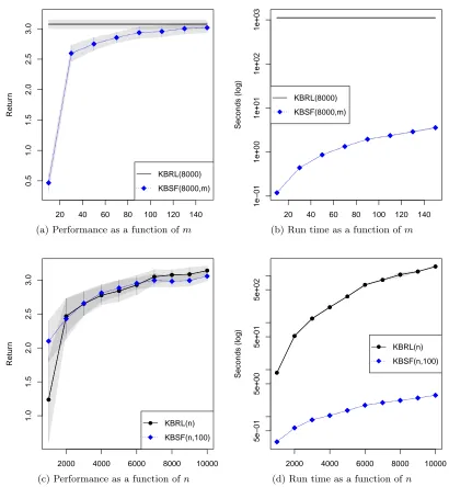
In Figure 3a and 3b we observe the effect of fixing the number of transitionsnand varying the number of representative states m. As expected, KBSF’s results improve asm → n. More surprising is the fact that KBSF has essentially the same performance as KBRL using models one order of magnitude smaller. This indicates that KBSF is summarizing well the information contained in the data. Depending on the values of n and m, such a compression may represent a significant reduction on the consumption of computational resources. For example, by replacing KBRL(8000) with KBSF(8000, 100), we obtain a decrease of approximately 99.58% on the number of operations performed to find a policy, as shown in Figure 3b (the cost of constructing KBSF’s MDP is included in all reported run times).
In Figures 3c and 3d we fix mand vary n. Observe in Figure 3c how KBRL and KBSF have similar performances, and both improve asnincreases. However, since KBSF is using a model of fixed size, its computational cost depends only linearly onn, whereas KBRL’s cost grows with n2nˆ, roughly. This explains the huge difference in the algorithms’s run times shown in Figure 3d.
4.2.2 Single and double pole-balancing (comparison with LSPI)
We now evaluate how KBSF compares to other modern reinforcement learning algorithms on more difficult tasks. We first contrast our method with Lagoudakis and Parr’s (2003) least-squares policy iteration algorithm (LSPI). Besides its popularity, LSPI is a natural candidate for such a comparison for three reasons: it also builds an approximator of fixed size out of a batch of sample transitions, it has good theoretical guarantees, and it has been successfully applied to several reinforcement learning tasks.
We compare the performance of LSPI and KBSF on the pole balancing task. Pole balancing has a long history as a benchmark problem because it represents a rich class of unstable systems (Michie and Chambers, 1968; Anderson, 1986; Barto et al., 1983). The objective in this problem is to apply forces to a wheeled cart moving along a limited track in order to keep one or more poles hinged to the cart from falling over. There are several variations of the task with different levels of difficulty; among them, balancing two poles side by side is particularly hard (Wieland, 1991). In this paper we compare LSPI and KBSF on both the single- and two-poles versions of the problem. We implemented the tasks using a realistic simulator described by Gomez (2003). We refer the reader to Appendix B for details on the problems’s configuration.
The experiments were carried out as described in the previous section, with sample transitions collected by a random policy and then clustered by the k-means algorithm. In both versions of the pole-balancing task LSPI used the same data and approximation architectures as KBSF. To make the comparison with LSPI as fair as possible, we fixed the width of KBSF’s kernelκaτ atτ = 1 and varied ¯τ in{0.01,0.1,1}for both algorithms. Also, policy iteration was used to find a decision policy for the MDPs constructed by KBSF, and this algorithm was run for a maximum of 30 iterations, the same limit used for LSPI.
20 40 60 80 100 120 140
0.5
1.0
1.5
2.0
2.5
3.0
Retur
n
KBRL(8000)
KBSF(8000,m)
(a) Performance as a function ofm
20 40 60 80 100 120 140
1e−01
1e+00
1e+01
1e+02
1e+03
Seconds (log)
KBRL(8000)
KBSF(8000,m)
(b) Run time as a function ofm
● ●
● ● ●
●
● ● ● ●
2000 4000 6000 8000 10000
1.0
1.5
2.0
2.5
3.0
Retur
n
● KBRL(n)
KBSF(n,100)
● ●
● ● ●
●
● ● ● ●
● ●
● ● ●
●
● ● ● ●
(c) Performance as a function ofn
● ●
● ●
● ● ●
● ● ●
2000 4000 6000 8000 10000
5e−01
5e+00
5e+01
5e+02
Seconds (log)
● KBRL(n)
KBSF(n,100)
● ●
● ●
● ● ●
● ● ●
● ●
● ●
● ● ●
● ● ●
(d) Run time as a function ofn
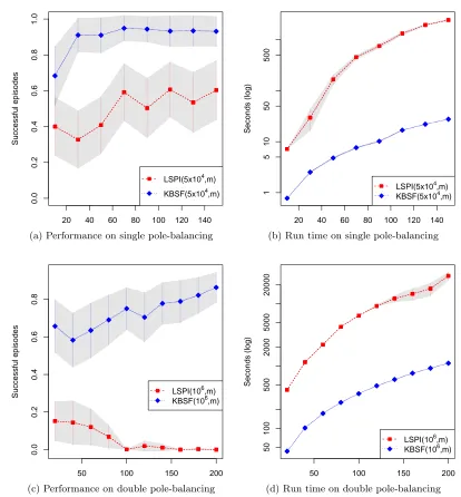
success rate of no more than 60% on the single pole-balancing task, as shown in Figure 4a. In contrast, KBSF’s decision policies are able to balance the pole in 90% of the attempts, on average, using as few asm= 30 representative states.
The results of KBSF on the double pole-balancing task are still more impressive. As Wieland (1991) rightly points out, this version of the problem is considerably more dif-ficult than its single pole variant, and previous attempts to apply reinforcement-learning techniques to this domain resulted in disappointing performance (Gomez et al., 2006). As shown in Figure 4c, KBSF(106, 200) is able to achieve a success rate of more than 80%. To put this number in perspective, recall that some of the test states are quite challenging, with the two poles inclined and falling in opposite directions.
The good performance of KBSF comes at a relatively low computational cost. A con-servative estimate reveals that, were KBRL(106) run on the same computer used for these experiments, we would have to wait for more than 6 months to see the results. KBSF(106, 200) delivers a decision policy in less than 7 minutes. KBSF’s computational cost also compares well with that of LSPI, as shown in Figures 4b and 4d. LSPI’s policy evaluation step involves the update and solution of a linear system of equations, which take O(nm2) and O(m3|A|3), respectively. In addition, the policy-update stage requires the definition of
π(ˆsak) for alln states in the set of sample transitions. In contrast, at each iteration KBSF only performs O(m3) operations to evaluate a decision policy andO(m2|A|) operations to update it.
4.2.3 HIV drug schedule domain (comparison with fitted Q-iteration)
We now compare KBSF with the fitted Q-iteration algorithm (Ernst et al., 2005; Antos et al., 2007; Munos and Szepesv´ari, 2008). Fitted Q-iteration is a conceptually simple method that also builds its approximation based solely on sample transitions. Here we adopt this algorithm with an ensemble of trees generated by Geurts et al.’s (2006) extra-trees algorithm. This combination, which we call FQIT, generated the best results on the extensive empirical evaluation performed by Ernst et al. (2005).
We chose FQIT for our comparisons because it has shown excellent performance on both benchmark and real-world reinforcement-learning tasks (Ernst et al., 2005, 2006). In all experiments reported in this paper we used FQIT with ensembles of 30 trees. As detailed in Appendix B, besides the number of trees, FQIT has three main parameters. Among them, the minimum number of elements required to split a node in the construction of the trees, denoted here byηmin, has a particularly strong effect on both the algorithm’s performance and computational cost. Thus, in our experiments we fixed FQIT’s parameters at reasonable values—selected based on preliminary experiments—and only varied ηmin. The respective instances of the tree-based approach are referred to as FQIT(ηmin).
20 40 60 80 100 120 140
0.0
0.2
0.4
0.6
0.8
1.0
Successful episodes
LSPI(5x10⁴,m)
KBSF(5x10⁴,m)
(a) Performance on single pole-balancing
20 40 60 80 100 120 140
1
5
10
50
500
Seconds (log)
LSPI(5x10⁴,m) KBSF(5x10⁴,m)
(b) Run time on single pole-balancing
50 100 150 200
0.0
0.2
0.4
0.6
0.8
Successful episodes LSPI(10
6
,m) KBSF(106,m)
(c) Performance on double pole-balancing
50 100 150 200
50
100
500
2000
5000
20000
Seconds (log)
LSPI(106,m) KBSF(106,m)
(d) Run time on double pole-balancing
is structured treatment interruption (STI), in which patients undergo alternate cycles with and without the drugs. Although many successful STI treatments have been reported in the literature, as of now there is no consensus regarding the exact protocol that should be followed (Bajaria et al., 2004).
The scheduling of STI treatments can be seen as a sequential decision problem in which the actions correspond to the types of cocktail that should be administered to a patient (Ernst et al., 2006). To simplify the problem’s formulation, it is assumed that RTI and PI drugs are administered at fixed amounts, reducing the actions to the four possible combinations of drugs: none, RTI only, PI only, or both. The goal is to minimize the viral load using as little drugs as possible. Following Ernst et al. (2006), we performed our experiments using a model that describes the interaction of the immune system with HIV. This model was developed by Adams et al. (2004) and has been identified and validated based on real clinical data. The resulting reinforcement learning task has a 6-dimensional continuous state space whose variables describe the overall patient’s condition.
We formulated the problem exactly as proposed by Ernst et al. (2006, see Appendix B for details). The strategy used to generate the data also followed the protocol proposed by these authors, which we now briefly explain. Starting from a batch of 6000 sample transitions generated by a random policy, each algorithm first computed an initial approximation of the problem’s optimal value function. Based on this approximation, a 0.15-greedy policy was used to collect a second batch of 6000 transitions, which was merged with the first.3 This process was repeated for 10 rounds, resulting in a total of 60000 sample transitions.
We varied FQIT’s parameter ηmin in the set {50,100,200}. For the experiments with KBSF, we fixed τ = ¯τ = 1 and varied m in{2000,4000, ...,10000} (in the rounds in which
m≥nwe simply used all states ˆsai as representative states). As discussed in the beginning of this section, it is possible to reduce KBSF’s computational cost with the use of sparse kernels. In our experiments with the HIV drug schedule task, we only computed theµ= 2 largest values of kτ(¯si,·) and the ¯µ= 3 largest values of ¯k¯τ(ˆsai,·) (see Appendix B.2). The
representative states ¯si were selected at random from the set of sampled states ˆsai (the
reason for this will become clear shortly). Since in the current experiments the number of sample transitions n was fixed, we will refer to the particular instances of our algorithm simply as KBSF(m).
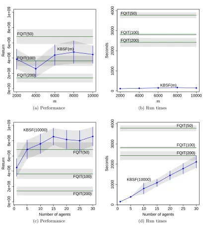
Before discussing the results, we point out that FQIT’s performance on the HIV drug schedule task is very good, comparable to that of Adams et al.’s (2004) approach, which uses a model of the task. FQIT’s results, along with KBSF’s, are shown in Figure 5. As shown in Figure 5a, the performance of FQTI improves whenηminis decreased, as expected. In contrast, increasing the number of representative statesmdoes not have a strong impact on the quality of KBSF’s solutions (in fact, in some cases the average return obtained by the resulting policies decreases slightly when mgrows). Overall, the performance of KBSF on the HIV drug schedule task is not nearly as impressive as on the previous problems. For example, even when using m= 10000 representative states, which corresponds to one sixth of the sampled states, KBSF is unable to reproduce the performance of FQIT with
ηmin = 50.
2000 4000 6000 8000 10000
0e+00
2e+08
4e+08
6e+08
8e+08
1e+09
m
Retur
n
FQIT(50)
FQIT(100)
FQIT(200)
KBSF(m)
(a) Performance
2000 4000 6000 8000 10000
0
1000
2000
3000
4000
m
Seconds
FQIT(50)
FQIT(100) FQIT(200)
KBSF(m)
(b) Run times
0 5 10 15 20 25 30
0e+00
2e+08
4e+08
6e+08
8e+08
1e+09
Number of agents
Retur
n
FQIT(50)
FQIT(100)
FQIT(200) KBSF(10000)
(c) Performance
0 5 10 15 20 25 30
0
1000
2000
3000
4000
Number of agents
Seconds
FQIT(50)
FQIT(100) FQIT(200)
KBSF(10000)
(d) Run times
On the other hand, when we look at Figure 5b, it is clear that the difference on the algorithms’s performance is counterbalanced by a substantial difference on the associated computational costs. As an illustration, note that KBSF(10000) is 15 times faster than FQTI(100) and 20 times faster than FQTI(50). This difference on the algorithms’s run times is expected, since each iteration of FQIT involves the construction (or update) of an ensemble of trees, each one requiring at least O(nlog(n/ηmin)) operations, and the improvement of the current decision policy, which is O(n|A|) (Geurts et al., 2006). As discussed before, KBSF’s efficiency comes from the fact that its computational cost per iteration is independent of the number of sample transitionsn.
Note that the fact that FQIT uses an ensemble of trees is both a blessing and a curse. If on the one hand this reduces the variance of the approximation, on the other hand it also increases the algorithm’s computational cost (Geurts et al., 2006). Given the big gap between FQIT’s and KBSF’s time complexities, one may wonder if the latter can also benefit from averaging over several models. In order to verify this hypothesis, we implemented a very simple model-averaging strategy with KBSF: we trained several agents independently, using Algorithm 1 on the same set of sample transitions, and then put them together on a single “committee”. In order to increase the variability within the committee of agents, instead of usingk-means to determine the representative states ¯sj we simply selected them uniformly at random from the set of sampled states ˆsai (note that this has the extra benefit of reducing the method’s overall computational cost). The actions selected by the committee of agents were determined through “voting”—that is, we simply picked the action chosen by the majority of agents, with ties broken randomly.
We do not claim that the approach described above is the best model-averaging strategy to be used with KBSF. However, it seems to be sufficient to boost the algorithm’s perfor-mance considerably, as shown in Figure 5c. Note how KBSF already performs comparably to FQTI(50) when using only 5 agents in the committee. When this number is increased to 15, the expected return of KBSF’s agents is considerably larger than that of the best FQIT’s agent, with only a small overlap between the 99% confidence intervals associated with the algorithms’s results. The good performance of KBSF is still more impressive when we look at Figure 5d, which shows that even when using a committee of 30 agents this algorithm is faster than FQIT(200).
4.2.4 Epilepsy-suppression domain (comparison with LSPI and fitted Q-iteration)
We conclude our empirical evaluation of KBSF by using it to learn a neuro-stimulation policy for the treatment of epilepsy. It has been shown that the electrical stimulation of specific structures in the neural system at fixed frequencies can effectively suppress the oc-currence of seizures (Durand and Bikson, 2001). Unfortunately, in vitro neuro-stimulation experiments suggest that fixed-frequency pulses are not equally effective across epileptic systems. Moreover, the long term use of this treatment may potentially damage the pa-tients’s neural tissues. Therefore, it is desirable to develop neuro-stimulation policies that replace the fixed-stimulation regime with an adaptive scheme.
was later validated through the deployment of a learned treatment policy on a real brain slice (Bush and Pineau, 2009). The associated decision problem has a five-dimensional continuous state space and highly non-linear dynamics. At each time step the agent must choose whether or not to apply an electrical pulse. The goal is to suppress seizures as much as possible while minimizing the total amount of stimulation needed to do so.
The experiments were performed as described in Section 4.2.1, with a single batch of sample transitions collected by a policy that selects actions uniformly at random. Specif-ically, the random policy was used to collect 50 trajectories of length 10000, resulting in a total of 500000 sample transitions. We use as a baseline for our comparisons the al-ready mentioned fixed-frequency stimulation policies usually adopted in in vitro clinical studies (Bush and Pineau, 2009). In particular, we considered policies that apply electrical pulses at frequencies of 0 Hz, 0.5 Hz, 1 Hz, and 1.5 Hz.
We compare KBSF with LSPI and FQIT. For this task we ran both LSPI and KBSF with sparse kernels, that is, we only computed the kernels at the 6-nearest neighbors of a given state (µ= ¯µ= 6; see Appendix B.2 for details). This modification made it possible to use m = 50000 representative states with KBSF. Since for LSPI the reduction on the computational cost was not very significant, we fixed m = 50 to keep its run time within reasonable bounds. Again, KBSF and LSPI used the same approximation architectures, with representative states defined by the k-means algorithm. We fixed τ = 1 and varied ¯
τ in {0.01,0.1,1}. FQIT was configured as described in the previous section, with the parameter ηmin varying in {20,30, ...,200}. In general, we observed that the performance of the tree-based method improved with smaller values forηmin, with an expected increase in the computational cost. Thus, in order to give an overall characterization of FQIT’s performance, we only report the results obtained with the extreme values of ηmin.
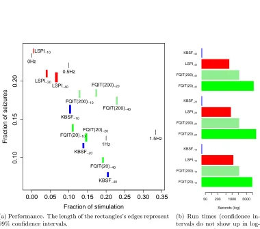
Figure 6 shows the results on the epilepsy-suppression task. In order to obtain different compromises between the problem’s two conflicting objectives, we varied the relative mag-nitude of the penalties associated with the occurrence of seizures and with the application of an electrical pulse (Bush et al., 2009; Bush and Pineau, 2009). Specifically, we fixed the latter at −1 and varied the former with values in {−10,−20,−40}. This appears in the plots as subscripts next to the algorithms’s names. As shown in Figure 6a, LSPI’s poli-cies seem to prioritize reduction of stimulation at the expense of higher seizure occurrence, which is clearly sub-optimal from a clinical point of view. FQIT(200) also performs poorly, with solutions representing no advance over the fixed-frequency stimulation strategies. In contrast, FQTI(20) and KBSF are both able to generate decision policies that are superior to the 1 Hz policy, which is the most efficient stimulation regime known to date in the clinical literature (Jerger and Schiff, 1995). However, as shown in Figure 6b, KBSF is able to do it at least 100 times faster than the tree-based method.
5. Incremental KBSF
0.00 0.05 0.10 0.15 0.20 0.25 0.30 0.35
0.10
0.15
0.20
Fraction of stimulation
Fr
action of seizures
0Hz
0.5Hz
1Hz
1.5Hz
FQIT(20)−40
FQIT(20)−10
FQIT(200)−40
FQIT(200)−10
KBSF−40
KBSF−20
KBSF−10
LSPI−40
LSPI−20
LSPI−10
FQIT(20)−20
FQIT(200)−20
(a) Performance. The length of the rectangles’s edges represent 99% confidence intervals.
FQIT(20)−10 FQIT(200)−10 LSPI−10 KBSF−10 FQIT(20)−20 FQIT(200)−20 LSPI−20 KBSF−20 FQIT(20)−40 FQIT(200)−40 LSPI−40 KBSF−40
Seconds (log) 50 200 1000 5000
(b) Run times (confidence in-tervals do not show up in log-arithmic scale)
even better. In this section we show how to build KBSF’s approximation incrementally, without ever having access to the entire set of sample transitions at once. Besides reducing the memory complexity of the algorithm, this modification has the additional advantage of making KBSF suitable for on-line reinforcement learning.
In the batch version of KBSF, described in Section 4, the matricesP¯aand vectors¯raare
determined using all the transitions in the corresponding setsSa. This has two undesirable consequences. First, the construction of the MDP ¯M requires an amount of memory of
O(ˆnm), where ˆn = maxana. Although this is a significant improvement over KBRL’s
memory usage, which is lower bounded by (minana)2|A|, in more challenging domains even
a linear dependence on ˆn may be impractical. Second, in the batch version of KBSF the only way to incorporate new data into the model ¯M is to recompute the multiplication
¯
Pa=K˙aD˙a for all actions afor which there are new sample transitions available. Even if we ignore the issue with memory usage, this is clearly inefficient in terms of computation. In what follows we present an incremental version of KBSF that circumvents these important limitations (Barreto et al., 2012).
We assume the same scenario considered in Section 4: there is a set of sample transitions
Sa ={(sak, rka,ˆsak)|k= 1,2, ..., na} associated with each action a∈ A, where ska,ˆsak ∈ S and rka ∈ R, and a set of representative states ¯S = {¯s1,s¯2, ...,sm¯ }, with ¯si ∈ S. Suppose
now that we split the set of sample transitions Sa in two subsets S1 and S2 such that
S1∩S2=∅andS1∪S2=Sa(we drop the “a” superscript in the setsS1 andS2 to improve clarity). Without loss of generality, suppose that the sample transitions are indexed so that
S1 ≡ {(sak, rak,ˆska)|k= 1,2, ..., n1}and S2 ≡ {(ska, rak,ˆsak)|k=n1+ 1, n1+ 2, ..., n1+n2 =na}.
LetP¯S1 and¯rS1 be matrixP¯aand vector¯racomputed by KBSF using only then
1transitions in S1 (if n1 = 0, we define P¯S1 =0 ∈ Rm×m and¯rS1 = 0 ∈Rm for all a ∈A). We want
to compute P¯S1∪S2 and ¯rS1∪S2 from P¯S1, ¯rS1, and S2, without using the set of sample
transitionsS1.
We start with the transition matrices P¯a. We know that
¯
pS1
ij =
Pn1
t=1k˙aitd˙atj=
Pn1
t=1
kτ(¯si, sat)
Pn1
l=1kτ(¯si, sal)
¯
kτ¯(ˆsat,¯sj)
Pm
l=1¯k¯τ(ˆsat,s¯l)
= Pn1 1
l=1kτ(¯si, sal)
Pn1
t=1
kτ(¯si, sat)¯k¯τ(ˆsat,sj¯)
Pm
l=1¯k¯τ(ˆsat,sl¯) .
To simplify the notation, define
zS1
i =
n1
X
l=1
kτ(¯si, sal), z S2
i =
n1+n2
X
l=n1+1
kτ(¯si, sal), and btij =
kτ(¯si, sat)¯kτ¯(ˆsat,¯sj)
Pm
l=1¯kτ¯(ˆsat,s¯l) ,
Now, defining bS2
ij =
Pn1+n2
t=n1+1b
t
ij, we have the simple update rule:
¯
pS1∪S2
ij =
1
zS1
i +z S2 i
bS2
ij + ¯p S1 ij z S1 i . (19)
We can apply similar reasoning to derive an update rule for the rewards ¯rai. We know that
¯
rS1
i =
1
Pn1
l=1kτ(¯si, sal) n1
X
t=1
kτ(¯si, sat)rta=
1
zS1
i n1
X
t=1
kτ(¯si, sat)rta.
Leteti = kτ(¯si, sat)rat, witht∈ {1,2, ..., n1+n2}. Then, ¯
rS1∪S2
i =
1
zS1
i +z S2 i
Pn1
t=1eti+
Pn1+n2
t=n1+1e
t i
= 1
zS1
i +z S2 i
zS1
i ¯r S1
i +
Pn1+n2
t=n1+1e
t i
.
DefiningeS2
i =
Pn1+n2
t=n1+1e
t
i, we have the following update rule:
¯
rS1∪S2
i =
1
zS1
i +z S2
i eS2
i + ¯r S1 i z S1 i . (20)
Since bS2
ij, e S2
i , and z S2
i can be computed based on S2 only, we can discard the sample
transitions in S1 after computingP¯S1 and¯rS1. In order to do that, we only have to keep the variables zS1
i . These variables can be stored in |A| vectors za ∈ Rm, resulting in a
modest memory overhead. Note that we can apply the ideas above recursively, further splitting the sets S1 and S2 in subsets of smaller size. Thus, we have a fully incremental way of computing KBSF’s MDP which requires almost no extra memory.
Algorithm 2 shows a step-by-step description of how to update ¯M based on a set of sample transitions. Using this method to update its model, KBSF’s space complexity drops fromO(ˆnm) toO(m2). Since the amount of memory used by KBSF is now independent of
n, it can process an arbitrary number of sample transitions (or, more precisely, the limit on the amount of data it can process is dictated by time only, not space).
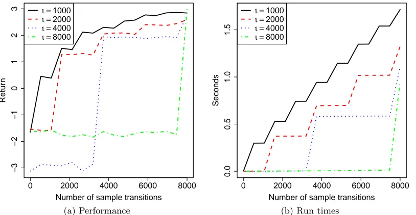
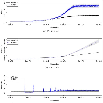
Instead of assuming thatS1 andS2 are a partition of a fixed data setSa, we can consider that S2 was generated based on the policy learned by KBSF using the transitions in S1. Thus, Algorithm 2 provides a flexible framework for integrating learning and planning within KBSF. Specifically, our algorithm can cycle between learning a model of the problem based on sample transitions, using such a model to derive a policy, and resorting to this policy to collect more data. Algorithm 3 shows a possible implementation of this framework. In order to distinguish it from its batch counterpart, we will call the incremental version of our algorithmiKBSF.iKBSF updates the model ¯M and the value functionQ¯ at fixed intervals
tm and tv, respectively. When tm =tv =n, we recover the batch version of KBSF; when
tm=tv = 1, we have a fully on-line method which stores no sample transitions.
Algorithm 3 allows for the inclusion of new representative states to the model ¯M. Using Algorithm 2 this is easy to do: given a new representative state ¯sm+1, it suffices to set