Learning Equivariant Functions with Matrix Valued Kernels

Learning Equivariant Functions with Matrix Valued Kernels

Marco Reisert [email protected]

Hans Burkhardt [email protected]

LMB, Georges-Koehler-Allee 52 Albert-Ludwig University 79110 Freiburg, Germany

Editor: Leslie Pack Kaelbing

Abstract

This paper presents a new class of matrix valued kernels that are ideally suited to learn vector valued equivariant functions. Matrix valued kernels are a natural generalization of the common notion of a kernel. We set the theoretical foundations of so called equivariant matrix valued kernels. We work out several properties of equivariant kernels, we give an interpretation of their behavior and show relations to scalar kernels. The notion of (ir)reducibility of group representations is transferred into the framework of matrix valued kernels. At the end to two exemplary applications are demonstrated. We design a non-linear rotation and translation equivariant filter for 2D-images and propose an invariant object detector based on the generalized Hough transform.

Keywords: kernel methods, matrix kernels, equivariance, group integration, representation theory,

Hough transform, signal processing, Volterra series

1. Introduction

In the last decade kernel techniques have gained much attention in machine learning theory. There is a large variety of problems which can be naturally formulated in a kernelized manner, ranging from regression and classification problems, over feature transformation algorithms to coding schemes. There is a large literature on this subject. We recommend Schoelkopf and Smola (2002) and Shawe-Taylor and Cristianini (2004) and references therein.

time-shifts and the action of the filter (in this case a linear convolution) commute. Equivariance is of high interest in signal-/image processing problems and geometrically related learning problems.

We give a constructive way to obtain kernels, whose linear combinations lead to equivariant functions. These kernels are based on the concept of group integration. Group integration is widely used for invariant feature extraction. For a introduction see Burkhardt and Siggelkow (2001). Re-cently Haasdonk et al. (2005) used group integration to get invariance in kernel methods.

The paper is organized as follows: In Section 2 we give a first motivation for our kernels by solving an equivariant regression problem. We give an illustrative interpretation of the kernels and present an equivariant Representer Theorem, which justifies our lax motivation from the beginning. Further we uncover a relation of our framework to Volterra theory. In Section 3 we give rules how to construct matrix kernels out of matrix kernels and give constraints how to preserve equivariance. Section 4 introduces the notion of irreducibility for kernels and show how the traces of matrix valued kernels are related to scalar valued kernels. Two possible application of matrix valued kernels are given in Section 5: a rotation equivariant non-linear filter and a rotation invariant object detector. Finally, Section 6 gives a conclusion and an outlook for future direction of research and applications.

2. Group Integration Matrix Kernels

In this section we propose the basic approach. After some preliminaries we give a first motivation for our idea. Then we give an interpretation of the proposed kernels and present an equivariant Representer Theorem.

2.1 Preliminaries and Notation

We consider compact (including finite), linear, unimodular groups

G

. A group representationρgis a

group homomorphism

G

7→L(

V

), where

V

is a finite dimensional Hilbert space usually called the representation space. Sometimes we write gx meaningρgx, where the patterns x∈

V

are always in

bold face. In the continuous case (

G

is a Lie group), the representation should also be continuous. In this case one can show that any representation of the group is equivalent to an unitary representation. For finite groups this statement also holds (for a proof see, for example, Lenz, 1990). So we can restrict ourselves with no loss of generality to unitary group representation, that is, alwaysρg−1 =

ρ†

g holds. We denote the Haar Integral (or Group Integral) by

R

G f(g) dg regardless whether we

deal with finite groups or continuous groups. Due to the unimodularity all reparametrizations are possible. For further reading on these topics we recommend Lenz (1990), Gaal (1973), Nachbin (1965), and Miller (1991); Schur (1968).

We want to learn functions f :

X

7→

Y

, where

X

,

Y

are finite dimensional Hilbert spaces. Tensor-or Kronecker products are denoted by ⊗. An equivariant function is a function fulfilling f(gx) = gf(x). The group actions on

X

and

Y

can be chosen such that they apply to the current application or problem. Inner products are denoted by h·|·iX, where the subscript indicates in which space the arguments are living. Due to the unitary group representation the inner product is invariant in the sensehgx1|gx2iX=hx1|x2iX. A scalar valued kernel is a symmetric, positive definite function k :

X

×

X

7→R_{fulfilling the Mercer property. More precisely, we use the term positive definite in}

the sense of semi-positive definiteness. If strict positive definiteness is forced, we make this explicit. We also assume invariance to group actions of

G

, that is, k(gx1,gx2) =k(x1,x2)for all g∈

G

. The

Z

k (isomorphic to the vector-valued RKHS of k), where the vector-valued coefficients live in

Y

,

that is,

Z

k={f(x) =∑ik(x,xi)ai|xi∈

X

,ai∈

Y

}.

We assume the reader is familiar with basics in kernel methods, tensor algebra and representa-tion theory.

2.2 Motivation

Our goal is to learn functions f :

X

7→

Y

from learning samples{(xi,yi)|i=1..n}in an equivariant

manner, that is, the function has to satisfy f(gx) =gf(x) for all g∈

G

, while f(xi) =yi should be

fulfilled as accurate as possible.

Due to the Representer Theorem by Kimeldorf and Wahba (1971) minimizer in

Z

k of arbitrary

risk functionals are of the form

f(x) =

n

∑

i=1

k(x,xi)ai, (1)

where the ai ∈

Y

are some vector valued coefficients, which have to be learned. To obtain an

equivariant behavior we pretend to present the training samples in all possible poses{(gxi,gyi)|i=

1..n, g∈

G

}. Since no pose g should be favored, the coefficients aiare not allowed to depend on g

explicitly, but they have to turn its pose according to the actions in the input space. And hence the solution has to look like

f(x) =

Z

G

n

∑

i=1

k(x,gxi)gaidg, (2)

where the integral ranges over the whole group

G

. As desired the following lemma holds

Lemma 2.1 Every function of form (2) is an equivariant function with respect to

G

.

Proof Due to the invariance of the kernel we have f(gx) =

Z

G

∑

_i k(x,g

−1_g0_x

i)g0aidg0,

and using the unimodularity of

G

we reparametrize the integral by h=g−1g0and obtain the desired result

f(gx) =

Z

G

∑

_i k(x,hxi)ghaidh=gf(x),

using the linearity of the group representation.

So we have a constructive way to obtain equivariant functions. Since we can exchange summa-tion with integrasumma-tion and the group acsumma-tion is linear we can rewrite (2) by

f(x) =

n

∑

i=1

Z

Gk(x,gxi)ρgdg

ai,

Proposition 2.2 Let K :

X

×

X

7→L(

Y

)for every x1,x2∈

X

be defined by

K(x1,x2) =

Z

Gk(x1,gx2)ρgdg,

where ρg∈L(

Y

) is a group representation and k is any symmetric,

G

-invariant function. The

following properties hold for a function above,

a) For every x1,x2∈

X

and g,h∈

G

, we have that

K(gx1,hx2) =ρgK(x1,x2)ρ†_h,

that is, K is equivariant in the first argument and anti-equivariant in the second, we say K is equivariant.

b) It holds K(x1,x2) =K(x2,x1)†_.

Proof To prove a) we just have to follow the reasoning in the proof of Lemma 2.1. For b) we use

the invariance and symmetry of k and the unimodularity of

G

and get

K(x1,x2) =

Z

Gk(g

−1_x1,x2)ρ gdg=

Z

Gk(x2,gx1)ρg−1 dg=K(x2,x1)

†_,

as asserted.

There are basically two ways to introduce matrix valued kernels in almost the same manner as for scalar-valued kernels. Following Aronszajn (1950) one can introduce a vector valued reproduc-ing kernel Hilbert space (RKHS) and then implicitly assume that there exists a kind of evaluation functional Kxin a certain Hilbert space of vector valued functions (for a more recent introduction

in the context of matrix valued kernels see Pontil and Micchelli (2004)). Basically the approach is as follows: by the Riesz Lemma there is a Kx such that hy|f(x)iY =hKxy|fi, where the inner

product on the right hand side works in the Hilbert space of vector valued functions. As the upper expression is linear in y one can define a linear operator in

Y

, the so called matrix valued kernel K(x1,x2)∈L(

Y

), by the following K(x1,x2)y := (Kx2y)(x1)equation.

A second possibility to introduce the notion of a matrix valued kernel is to demand the existence of a feature mapping into a certain feature space. For example for scalar valued kernels this is done by Shawe-Taylor and Cristianini (2004). For matrix valued kernels the feature space can be identified as the tensor product space of linear mappings on

Y

times an arbitrary high dimensional feature space.

Both, the RKHS approach and the feature space approach are equivalent due to a generalized Mercer Theorem. We decided for the latter alternative. It is more appropriate for our purposes, because we can explicitly access the structure of the induced feature space.

Definition 2.3 (Matrix Valued Kernel) A function K :

X

×

X

7→L(

Y

) is called a matrix valued kernel if there is a sesqui-linear form such that for all x1,x2∈

X

K(x1,x2) =hΨ(x1)|Ψ(x2)iH

The elements of the feature-space

H

can be imagined as L(

Y

)-valued or matrix-valued vectors, just elements of

F

⊗L(

Y

). Actually it carries the structure of a L(

Y

)-bimodule. A module is a generalization of a vector space where the field elements are replaced by noncommutative ring elements. For a bimodule right and left multiplication are defined (see, for example, R. G. Douglas, 1989). Additionally we have to define the adjoint for the ring-elements L(

Y

), which simply turns out to be the adjoint of the linear mapping. The connection of the feature space representation to the RKHS of Aronszjan is simple. Similarly to the case of the scalar kernels, the evaluation functionals Kx have to be associated with the elements Ψ(x) living in the feature space

F

⊗L(

Y

). In the

RKHS the functions are represented by linear combinations∑_iKxiai; in the feature space the linear

combination takes the form∑_iΨ(xi)ai which is an element of

F

⊗

Y

. The space

F

⊗

Y

carries

the structure of a L(

Y

)-left module, because multiplication from the left by elements in L(

Y

)is allowed. Note that this a fundamental difference to scalar kernels. In the case of scalar kernels the representation of functions and the evaluation functionals live in the same space. For matrix kernels it is different. The evaluation functional are elements of a L(

Y

)-bimodule or explicitly

F

⊗L(

Y

); the functions are elements of the L(

Y

)-left module

F

⊗

Y

.

Remark 2.4 In Definition 2.3 the matrix-valued inner product in

H

also induces a scalar inner product by the trace tr(hΨ|Ψ0_i

H)and it indeed holds that tr(hΨ|ΨiH)≥0 for allΨ6=0. Hence the

space

H

is naturally attached with a (semi-)norm||Ψ||=ptr(hΨ|Ψi_H).

Theorem 2.5 (GIM-kernels) If the function k is a scalar kernel, then the function K given in

Proposition 2.2 is a matrix valued kernel. We call this kernel a Group Integration Matrix kernel or short GIM-kernel.

Proof To show this, we give the feature mappingΨ by the use of the feature mappingΦ corre-sponding to the scalar kernel k and show that the GIM-kernel can be written as a positive matrix valued inner product in the new feature space

H

=

F

⊗L(

Y

). LetΨbe given by

Ψ(x) = p1 µ(

G

)

Z

GΦ(gx)⊗ρgdg,

where µ(

G

) =R

Gdg is the volume of the group. The matrix valued inner product in

H

is given by

the rule

hΦ1⊗ρ1|Φ2⊗ρ2iH :=ρ†1ρ2hΦ1|Φ2iF

and its linear extension, that is, it is a sesqui-linear mapping of type

H

×

H

7→L(

Y

). And the so defined product is indeed positive. Any Ψ∈

H

can be written as a sum (integral) of Kronecker productsΨ=∑_iΦi⊗ρi. So for anyΨ∈

H

and any y∈

Y

we have

hy|hΨ|Ψi_HyiY =

∑

i,j

hΦi|ΦjiFhρiy|ρjyiY =

∑

i,j

ki jhρiy|ρjyiY =

∑

i,j

ki jhyi|yjiY ≥0

is positive, because the matrix ki j is positive definite by the Mercer property of k.

Using the above rule for the inner product we can compute

hΨ(x1)|Ψ(x2)i_H = 1 µ(

G

)

Z

G2

hΦ(gx1)⊗ρg|Φ(hx2)⊗ρhiH dg dh

= 1

µ(

G

)

Z

G2

Inserting the scalar kernel k and reparametrizing by g0=g−1h gives

hΨ(x1)|Ψ(x2)i_H = 1 µ(

G

)

Z

G2

k(x1,g0x2)ρg0 dg0dh= Z

Gk(x1,gx2)ρgdg=K(x1,x2)

which is the desired result.

2.3 Examples and Interpretation of Equivariant Kernels

To get more intuition how equivariant kernels, not necessarily GIM-kernels, behave, we want to sketch how such kernels can be interpreted as estimates of the relative pose of two objects. First we consider the probably most simple equivariant kernel, the complex hermitian inner product itself. The group U(1) consists of all complex numbers of unit length. If we define the representation of U(1)acting on theCn _{by a simple scalar multiplication with a complex unit number, then the}

ordinary inner product is obviously equivariant, that is

hg1x1|g2x2i=heiφ1_x1|eiφ2_x2i=eiφ1_hx1|x2ie−iφ2 _=g

1hx1|x2ig†₂.

The absolute value of hx1|x2i can be interpreted as some kind of similarity. But how one should interpret the complex phase of hx1|x2i? Therefore consider the distance J(φ) =||x1−eiφx2|| for different values ofφ. It is easy to show that J is minimal ifφis chosen according to eiφ= hx1|x2i

|hx1|x2i|. Thus, the phase of the inner product carries information about the relative pose of the two objects. Actually this result can be generalized for equivariant kernels. Assume that we want to align the featuremapsΨ(x1)andΨ(x2)of an equivariant kernel optimally with respect to the group

G

, that

is, we try to minimize

J(g) =||Ψ(x1)−Ψ(gx2)||2,

Reformulating the objective leads to maximizing the trace

J0(g) =tr(K(x1,x2)ρ†_g+ρgK(x2,x1)),

Let us assume that the group representation is surjective, that is, for any unitary matrix there is a g∈

G

such thatρgis identical to this matrix. Then we can use the Singular Value Decomposition (SVD)

of the kernel to get the optimal solution. Let K(x1,x2) =VΣW the SVD, then one can show that

ρg∗=VW gives the optimal alignment, where J0takes J0(g∗) =2tr(Σ)in the optimum. Interpreting this result, we can say that the sum of the singular values of a equivariant kernel expresses the similarity of the two given objects, while the unitary parts U and V contain information about the relative pose of the objects. And in fact, if x1=g0x2, then g∗=g0holds.

We want to demonstrate the proposed behavior with another example. Consider the finite group of cyclic translations Cn acting on the n dimensional vector space

X

=Cn. The group elements

gk with k=0, . . . ,n−1 act on this space by [ρgkx]l := [x](l−k) mod n. This is just one particular

representation of Cn. Another representation for example acts by scalar multiplications ρ0gky :=

and whose output space is

Y

=C_{with the representation}ρ0

g. One can choose

Y

one dimensional

becauseρ0_gjust acts by scalar multiplications. The GIM-kernel K :

X

×

X

7→C_{is given by}

K(x1,x2) =

n−1

∑

k=0

hx1|ρgkx2ie

i2_nπk_.

To interpret the behavior of K and understand with respect to which properties the objects are aligned we consider the feature Ψ(x). Having a closer look the feature is nothing else than the first coefficient of a discrete Fourier expansion of x. Thus, the kernel is just the product of the first coefficients of object x1 with the complex conjugate coefficient of x2. Consequently, the unitary

part of the kernel, the complex phase, represents the relative phase of the first Fourier modes of the objects. The alignment with respect to those is a very common procedure in image processing applications to obtain complete invariant feature sets for the cyclic translation group Cn or other

abelian groups like the two dimensional rotations SO(2)(see, for example, Canterakis, 1986). The considerations get more intricate when non-abelian groups are considered. For 3D rotations this subject is discussed by Reisert and Burkhardt (2005) in more detail.

2.4 Equivariant Representer Theorem

In the beginning of this section we motivated our approach by pretending to present training patterns in all possible poses, where the pose of a target is implicitly turned by letting the group act on the regression coefficients. We did not clarify whether this is the optimal solution to obtain an equivariant behavior. Are there other possible solutions which are more general but also equivariant? It is easy to check that the subspace

E

⊂

Z

kof equivariant functions is a linear subspace. The

projectionΠ_E onto this subspace is given by

(ΠEf)(x) = 1 µ(

G

)

Z

G

g−1f(gx)dg. (3)

This projection operator is the core of the construction principle presented in this work. In classical invariant theory this operator is also known as the Reynolds operator (Mumford et al., 1994).

Lemma 2.6 The projectionΠ_E of (1) admits the proposed representation given in (2).

Proof Applying the projection on (1) yields

(ΠEf)(x) = 1

µ(

G

)

Z

G

n

∑

i=1

k(gx,xi)g−1aidg=

1 µ(

G

)

Z

G

n

∑

i=1

k(x,g−1xi)g−1aidg

= 1

µ(

G

)

Z

G

n

∑

i=1

k(x,hxi)haidh,

where we used the substitution h=g−1.

which are based on scalar kernels (as introduced in Eq. (1)) look in feature space. As already men-tioned the evaluation functionals and the representations of the functions live in different spaces. The function of form (1) has the following representation f(x) =hΦ(x)⊗I_Y|ΨfiH. The matrix

IY ∈L(

Y

)denotes the identity matrix on

Y

. The corresponding feature-space representationΨfis

an element of the contracted feature-space

F

⊗

Y

, a L(

Y

)-left-module. This is easy to see when you think of

F

⊗

Y

as vectors whose components itself are column vectors. These column vectors only admit multiplication by matrices from the left as we know from ordinary matrix calculus. The feature space representation of the function is obviously of the formΨf=∑iΦ(xi)⊗ai, where the ai are vector-valued expansion coefficients. The naturally induced scalar-valued inner product in

this space is given by

hΦ⊗a|Φ0⊗a0iF⊗Y =hΦ|Φ0iFha|a0iY. (4) The projection operatorΠE as defined in Eq. (3) acts directly on the functions f. To show that

ΠEis unitary we must examine how it acts on the feature space representation. Therefore, we define the group action on

F

⊗

Y

g(Φ(x)⊗a):=Φ(g−1x)⊗(g−1a). (5)

By the use of this we define a new operator ˜Π_E acting on

F

⊗

Y

and show that it corresponds to

ΠE and that it is unitary with respect to the inner product given in Eq. (4).

Proposition 2.7 If ˜ΠE is given by ˜

ΠEΨf:=

1 µ(

G

)

Z

GgΨfdg

then ˜ΠEΨf=ΨΠEfholds and ˜ΠE is a unitary projection.

Proof LetΨf=∑iΦ(xi)⊗aiand correspondingly f(x) =∑ni=1k(x,xi)ai. Then

(Π_Ef)(x) = 1

µ(

G

)

Z

G

n

∑

i=1

k(gx,xi)g−1ai dg=

1 µ(

G

)

Z

G

hΦ(gx)⊗ρg|ΨfiH

= hΦ(x)⊗I_Y| 1

µ(

G

)

Z

GgΨfiH =hΦ(x)⊗IY|Π˜EΨfiH

this yields ˜Π_EΨf =ΨΠEf. The operator ˜ΠE is obviously a projection, because ˜Π2_E =Π˜E. The

unitarity is due to unimodularity of the group. It is easily proved by showing that ˜Π_E is hermitian with respect to the inner product in Eq. (4).

In conclusion, due to the unitartity the projection ˜ΠE gives the best equivariant approximation of an arbitrary function in

Z

k. The space of equivariant function

E

is nothing else than the space of fix

points with respect to the group action defined in Eq. (5), that is

E

={Ψ∈

F

⊗

Y

|∀g∈

G

: gΨ=Ψ}. The proof of the following theorem is similar to the proof given in Schoelkopf and Smola (2002) for the general Representer Theorem. Note that we allow coupling between the training samples.

Theorem 2.8 (Equivariant Representer Theorem) Let Ω:R+ _7→R _{be a strictly monotonically}

increasing function and c :(

X

×

Y

×

Y

)n_{7→Ra loss function. Then each equivariant minimizer} f∈

Z

kof

is of the form

f(x) =

Z

G

n

∑

i=1

k(x,gxi)gaidg,

Proof We can decompose a function f∈

Z

korthogonally (in the sense of the inner product given in

(4)) into a part in the span of

{Φ(xi)⊗y∈

F

⊗

Y

|i=1..n,y∈

Y

}

and its orthogonal complement;

f(x) = f_||(x) +f⊥(x).

We know by construction that f⊥(xi) =0 for all i=1..n. Every equivariant function in

Z

k is a

projection of the formΠ_Ef. Considering the projection of the decomposition

(Π_Ef)(x) = (Π_Ef||)(x) + (ΠEf⊥)(x)

we also know that the second term(ΠEf⊥)(xi) =0 vanishes for all training samples. Thus the loss

function in R(Π_Ef)stays unchanged if one neglectsΠ_Ef⊥. By Lemma 2.6 we know thatΠEf||is of

the proposed form

ΠEf||= Z

G

n

∑

i=1

k(x,gxi)gaidg.

Due to the orthogonality we also know

||Π_Ef||2 = ||Π_Ef_||||2+||Π_Ef⊥||2

and henceΩ(||Π_Ef||2_)≥Ω_(||Π

Ef||||2). And thus for fixed values of aiwe get R(ΠEf)≥R(ΠEf||),

so we have to chooseΠEf⊥=0 to minimize the objective. As this also has to hold for the solution,

the theorem holds.

Note that the above theorem makes only statements for vector valued function spaces induced by a scalar kernel. There are also matrix valued kernels that are not based on a scalar kernels, that is, GIM-kernels are not the only way to obtain equivariant kernels. In Section 4 we will work out that one important class of equivariant kernels are GIM-kernels, namely those kernels whose corresponding group representation is irreducible.

2.5 Non-Compact Groups and Relation to Volterra Filters

In this work we consider compact unimodular groups. This is indeed very restrictive. Demand-ing that the functions f(g) =k(x1,gx2)are all functions of compact support, it seems possible to

generalize our theory for non-compact groups.

generalized non-linear convolutions. The Volterra theory states that a nonlinear system, that maps a function x defined on the time line on a function f in an equivariant manner, can be modeled as infinite sums of multidimensional convolutions of increasing order

[f(x)]t =h0+ Z

g∈G

h1(g)[gx]tdg+

Z

g∈G Z

g0_∈G

h2(g,g0)[gx]t[g0x]t dgdg0+...,

where[x]t denotes the value of x at time t and

G

is the group of time-shifts. In fact, Volterra series

of degree n can be modeled with polynomial matrix kernels of degree n, that is, the scalar basis kernel is k(x1,x2) = (1+hx1|x2i)n. In other words, the RKHS of the induced matrix kernel is the

space of n-th order Volterra series. Using the exponential kernel k(x1,x2) =eλhx1|x2i the RKHS is

actually the space of infinite degree Volterra series. For higher order polynomial kernels or even exponential kernels a kernelization is quite useful, because the run-time is linear in the number of training samples instead of proportional to the size of the induced feature space. There is already work by Dodd and Harrison (2003) which proposes a similar kernelized version of Volterra theory, but our theory is much more general. Our work tries to give a kernelized generalization of Volterra theory for arbitrary unimodular groups from a machine learning point of view.

3. Constructing Kernels

Similar to scalar valued kernels there are also several building rules to obtain new matrix and scalar valued kernels from existing ones. Most of them are similar to the scalar case, but there are also ’new’ ones. In particular, the rule for building a kernel out of two kernels by multiplying them splits into two rules, either using the tensor product or the matrix product.

Proposition 3.1 (Closure Properties) Let K1:

X

×

X

7→L(

Y

)and K2:

X

×

X

7→L(

Y

0)be matrix

valued kernels and A∈L(

V

,

Y

)with full row-rank, then the following functions are kernels.

a) Let

Y

=

Y

0. K(x1,x2) =K1(x1,x2) +K2(x1,x2)

b) K(x1,x2) =A†K1(x1,x2)A

c) K(x1,x2) =K1(x1,x2)⊗K2(x1,x2)

d) Let

Y

=

Y

0. If for all x∈

X

, K1(x,x) and K2(x,x) commute, then the matrix product

K(x1,x2) =K1(x1,x2)K2(x1,x2)is a kernel.

e) K(x1,x2) =K1(x1,x2)†

f) k(x1,x2) =tr(K1(x1,x2))

Proof We omit proofs for a) and b) since the reasoning directly translates from the scalar case. To

show c) for matrix kernels we give the corresponding feature-maps in terms of the already known feature-mapsΨ1,Ψ2for kernel K1and K2. From ordinary tensor calculus we know that

hΨ1⊗Ψ2|Ψ01⊗Ψ20iK1⊗K2 =hΨ1|Ψ

0

1iK1⊗ hΨ2|Ψ

so the new feature-map for the tensor-product kernel c) is obviouslyΨ=Ψ1⊗Ψ2. The positivity

is also given, since the tensor product of two positive definite matrices is again positive definite. For d) the feature-map is actually the same as for c), but we define a different inner product by

hΨ1⊗Ψ2|Ψ01⊗Ψ20iK1K2:=hΨ1|Ψ

0

1iK1hΨ2|Ψ

0 2iK2,

which extends uniquely to the whole space and is well defined. Since we assume that the diagonal kernels K1(x,x)and K2(x,x)commute, the positive definiteness is also given, because the

eigenval-ues of the matrix product are just the products of the positive eigenvaleigenval-ues of its factors. The proof of e) is trivial. For the proof of statement f), we only have to recall Remark 2.4, where we mentioned that the trace of a positive matrix valued product is an ordinary positive scalar inner product.

Let us have a look how such rules can be applied to equivariant kernels and under what circum-stances equivariance is preserved. Rule a) can be applied if K1and K2have the same transformation

behavior, meaning that the underlying group representations are identical. Rule b) preserves equiv-ariance if the matrix A is unitary. One can see this by redefining the group representation on

Y

by

ρ0

g=A†ρgA. Sinceρ0gis again an unitary representation, K is an equivariant kernel. Rule c) can also

be used to construct equivariant kernels. Supposing an equivariant kernel K1and an invariant scalar

kernel k in sense that k(x1,gx2) =k(x1,x2)for all g∈

G

, then rule c) implies that K=K1⊗k=K1k

is also a kernel and in fact equivariant. But how can we construct an invariant kernel k. The simplest approach is to use invariant features, but our framework also offers two possibilities. A GIM-kernel based on the trivial representation (justρg=1) is obviously invariant (this special case covers the

approach proposed by Haasdonk et al., 2005). Another possibility is to use rule d) and f) to obtain an invariant kernel. But therefore we have to force the kernel to be normal, that is, the kernel K must always commute with its transpose K†.

Lemma 3.2 If K is a normal equivariant kernel, then k=tr(K†K) is an invariant kernel in the following sense k(x1,gx2) =k(g0x1,x2) =k(x1,x2)for all g,g0∈

G

.

Proof Since K is normal K(x,x)commutes with its transpose and hence K†K is a kernel by rule d). By rule f) we know that tr(K†K)is a kernel. The invariance of the trace

k(x1,gx2) =tr((Kρ†g)†Kρ†g) =tr(ρgK†Kρ†g) =tr(K†K) =k(x1,x2)

proves invariance of the kernel.

4. Irreducible Kernels

fully occupied matrix. To formalize this more precisely we introduce the notion of irreducibility for matrix kernels, which should cover the intuition that a kernel cannot be decomposed in a more simple, more diagonal kernel.

Definition 4.1 A kernel K(x1,x2)∈L(

Y

) is reducible if there is a nonempty subspace

W

⊂

Y

, such that for every y∈

W

and for every x1,x2∈

X

, we have K(x1,x2)y∈

W

, otherwise the kernel

is called irreducible.

This definition is very close to the notion of irreducibility for group representations. This notion plays the central role in the harmonic analysis of groups (see Miller, 1991). A group representation

ρg∈L(

V

)is called reducible if there exists a nonempty subspace

W

⊂

V

such that for all w∈

W

also ρgw∈

W

. Then

W

is called a invariant subspace. If a representation is not reducible it is

called irreducible. For all abelian groups the irreducible representations are very simple and all one-dimensional. They are just the complex numbers of unit length. Most of the readers may know them as Fourier transformations. For example, for the group of two dimensional rotation SO(2), they are justρ(gl)=eilφ. The invariant subspace on whichρ(gl) is acting is justC, a one dimensional vector

space. Suppose a given function on the circle, then the lth component of the Fourier representation of this function is exactly the representation space on which the representation ρ(gl) is acting on.

For abelian groups the basis function on which the irreducible representation are working have the same formal appearance as the irreducible representations itself which might be confusing. For non-abelian groups it is different. Consider the group of three dimensional rotations SO(3). The corresponding irreducible representations are the so called D-Wigner matrices which are not one dimensional anymore. They are matrices of increasing sizeρ(gl)∈C(2l+1)×(2l+1). They act obviously

on 2l+1 dimensional vector spaces. For a given function defined on a three-dimensional sphere the expansion in the invariant subspaces is the so called Spherical Harmonic expansion which is also sometimes called the Fourier representation of the 2-Sphere. One may call harmonic analysis the generalization of Fourier theory to non-abelian groups.

If an equivariant kernel transforms by an irreducible representation, then it can be deduced that also the kernel itself is irreducible. But the opposite direction is not true in general, otherwise any equivariant kernel would be a GIM-kernel. We will later discuss this in more detail. But first two basic properties.

Lemma 4.2 If the representationρof a strictly positive definite, equivariant kernel K is irreducible then K is also irreducible.

Proof Assume that K is reducible, then there is a subspace

W

⊂

Y

, such that y∈

W

⇒K(x1,x2)y∈

W

. Sinceρis irreducible, we can choose y∈

W

such that there exists a g withρgy=w+w⊥∈

W

⊕

W

⊥. But we also know that K(x1,g−1x2)y=K(x1,x2)ρgy∈

W

. In particular, we can choose x1=x2=x. Due to the reducibility of K and the regularity (because of strictly pd) of K(x,x), we

know that 06=K(x,x)w⊥∈

W

⊥_{and hence K(x,x)ρ}

gy∈/

W

. Contradiction!

Corollary 4.3 Any GIM-kernel K can be decomposed in a direct sum of irreducible GIM-kernels

associated with its irreducible representations.

Proof Letρbe the representation of the GIM-kernel. Since anyρcan be decomposed in a direct sumρ=ρ(1)_⊕...⊕ρ(n)_{, we directly see that}

K=K1⊕..⊕Kn,

where Kl(x1,x2) =R_Gk(x1,gx2)ρ(gl)dg. And the Kl are irreducible due to Lemma 4.2.

By the Peter-Weyl-Theorem (Gaal, 1973) we know that the entries of the irreducible representa-tions of a compact group

G

form a basis for the space of square-integrable function on

G

. We also know that the entries of the representations are orthogonal with respect to the canonical dot-product. The following Lemma is based on that.

Lemma 4.4 If the representationρof an equivariant kernel K is irreducible then K is a GIM-kernel.

Proof We define the corresponding scalar kernel by

k= n

µ(

G

)tr(K),

where n is the dimensionality of the associated group representation. Then

Z

Gk(x1,gx2)ρgdg=

n µ(

G

)

Z

Gtr(K(x1,x2)ρ

† g)ρgdg.

By the orthogonality relations for irreducible group representations we know that

n µ(

G

)

Z

Gtr(K(x1,x2)ρ

†

g)ρgdg=K(x1,x2).

It seems that we should concentrate on the irreducible representations of the considered group, and this is indeed the canonical way. Any scalar kernel can be written in terms of its irreducible GIM-kernel expansion.

Proposition 4.5 Let k be a scalar kernel, then

k(x1,x2) =tr(K(x1,x2)),

where K=K1⊕K2⊕...is the direct sum of its irreducible GIM-kernels as given in Corollary 4.3 Proof Due to the Peter-Weyl-Theorem we can expand the scalar kernel in terms of the irreducible

representation of

G

, where the expansion coefficients are by definition the corresponding GIM-kernels.

k(x1,gx2) =

∞

∑

l=0

where Kl(x1,x2) =R_Gk(x1,gx2)ρ(gl)dg. And hence we have

k(x1,gx2) =

∞

∑

l=0

tr(Kl(x1,gx2)) =tr(K1(x1,gx2)⊕K2(x1,gx2)⊕...) =tr(K(x1,gx2)),

which proves the statement.

Hence we have a one-to-one correspondence between the scalar basis kernel k and the GIM-kernels Klformed by the irreducible group representationsρ(gl). So we have for GIM-kernels always

the duality between the matrix- and scalar-valued kernels. For Non-GIM-kernels this one-to-one correspondence does not hold.

4.1 Non GIM-kernels

There is another very simple way to construct equivariant kernels. For example assume that

X

=

Y

then K(x1,x2) =|x1ihx2|is obviously an equivariant kernel. This kernel may be seen as the matrix-valued analogon to the linear scalar-matrix-valued kernel k(x1,x2) =hx2|x1iX and indeed k=tr(K)holds. Note that it is in general not possible to reconstruct K from tr(K), this is only possible for GIM-kernels by Proposition 4.5. Such a non GIM-kernel can be easily obtained by the construction principle from above. But how to check whether a kernel is a GIM-kernel or not?

Corollary 4.6 Let K be an irreducible equivariant kernel and let its corresponding representation

be reducible, then K is not a GIM-kernel.

Proof Assume K is of GIM-type then by Corollary 4.3 it is reducible. Contradiction!

This statement is the counterpart to Lemma 4.4, which says that if the group-action is irreducible we know that we have a GIM-kernel.

The simple kernel K(x1,x2) =|x1ihx2|is not of practical value, because regression functions which are built out of it are always proportional their input. So one needs clever feature-maps to get useful kernels.

4.2 Kernel Response for Symmetric Patterns

GIM-kernels provide an intrinsic mechanism to cope with symmetric patterns. A pattern x∈

X

is called

U

-symmetric if there is a subgroup

U

of

G

such that for all u∈

U

we have ux=x. To

characterize the kernel response for such patterns we define a linear unitary projection on the space of

U

-symmetric patterns as follows

πUx := 1 µ(

U

)

Z

Ugx dg. (6)

The operatorπUis a unitary projection due to the same arguments as used in the proof of Proposition 2.7. Using this operator we can state the following

Lemma 4.7 Let K be a GIM-kernel. If x1is

U1

-symmetric and x2is

U2

-symmetric then

Proof Let

G

/

U

the quotient group. If x2is

U2

-symmetric then

K(x1,x2) = 1 µ(

G

)

Z

G

k(x1,gx2)ρgdg=

1 µ(

G

)

Z

G/U2 Z

U2

k(x1,gux2)ρgudu dg

= 1

µ(

G

/

U2

)

Z

G/U2

k(x1,gx2)dg

1 µ(

U2

)

Z

U2

ρudu

| {z }

πU2

.

Asπ_U is a projection and thusπ2_U =π_U we can insert aπ_U2 in the last line from above for free and reverse the whole computation an obtain K(x1,x2) =K(x1,x2)πU2. If x1is

U1

-symmetric the reasoning is very similar. Due to the unimodularity of the group and its subgroups it is no problem to exchange g and u in the last expression from the first line. Hence, we can use the same arguments as for theπ_U2-symmetry.

Assume now we have a trained function f(x)composed as a linear combination of GIM-kernels. What is the response of f(x)if x is

U

-symmetric. Due to Lemma 4.7 it is obvious that f(x)is also

U

-symmetric and the symmetrization is obtained via the operator defined in Eq. (6). This behavior is reasonable, because there is no reason why the output should violate the symmetry if the input does not spend information beyond. For example, if the output space

Y

is a space of probability distributions the idea of symmetrization viaπU is a good idea. Because, if we are uncertain about the original pose of an input object due to symmetry, we should vote for all possible outputs allowed by the symmetry in a additive manner. And the operatorπUactually works this way.

Now let us consider the opposite view. Suppose we want to build a function that maps a

U

-symmetric input x0 to a not symmetric output y0, which is obviously an ill-posed problem. How

does the function behave? We are not able to make a general statement, because it depends on the learning algorithm applied. But to get an intuition consider the function f(x) =K(x,x0)y0, which essentially behaves as desired, if K(x,x)∝I_Y. By Lemma 4.7 we know that f(x) =K(x,x0)(πUy0)

holds, thus the function behaves as if the desired output was symmetrized beforehand.

5. Applications

for each pixel in the Image

map in a rotation− equivariant manner project on

local basis

reconstruct patch

assemble Image

PSfrag replacements

xz

z

Image I Image F(I)

[xz]n ∑n[f(xz)]n[bz]n

Map in an equivariant manner

f

f(xz)

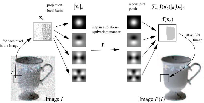
Figure 1: The workflow of the rotation equivariant filter for the example of image denoising.

5.1 Equivariant Kernels for 2D Rotations

In both experiments we want to learn functions f :

X

7→

X

, where

X

is the space of functions defined on the unit circle. The irreducible representations of 2D-rotations are einφand the irreducible subspaces correspond to the Fourier representation of the function. Hence in Fourier representation the GIM-kernel is a diagonal kernel with entries

Kn(x1,x2) =

Z 2π 0

k(x1,gφx2)einφdφ (7)

on the diagonal. Discrete approximations of this integral can be computed quickly by a Fast Fourier Transform (FFT). Assuming k is a dot-product kernel k(hx1|x2iX), then a kernel evaluation looks as follows: Compute the cross-correlation c(φ) =hx1|gφx2iX using the FFT, apply the nonlinearity k(c(φ)) and transform it back into Fourier domain Kn=R₀2πk(c(φ))einφ dφ. If the patterns are

already in Fourier domain, we need two FFT per kernel evaluation. This approach is used in the second experiment.

The probably most simple non-linear scalar kernel is k(x1,x2) =hx1|x2i2

X. Using this kernel as a scalar base kernel the matrix-valued feature space looks very simple. The feature map is given by

[Ψ(x)]nl ∝[x]−l [x]l+n, (8)

where[x]l denotes lth component of the Fourier representation of x. The induced matrix valued

bilinear product in this space is the ordinary

Kn(x1,x2) =

∑

l

[Ψ(x1)]nl [Ψ(x2)]∗nl.

5.2 A Rotation Equivariant Filter for Images

For convenience we represent a 2D gray-value image I in the complex plane, where we denote the gray value at point z∈C_{by Iz. The idea is to learn a rotation-equivariant function f :}

X

_7→

X

_{, which}

maps each neighborhood xz∈

X

of a pixel z onto a new neighborhood f(xz)∈

X

with properties

given by learning samples. The neighborhood is represented by projections on local basis functions [bz]n=zne−λ|z|

2

for n=0, . . . ,N−1. This basis is actually a orthogonal basis with respect to the standard inner product. In Figure 1 the appearance of the basis is depicted. In particular, for each pixel z0the inner product

[xz0]_n=hI_z−z0|zne−λ|z| 2

i=

∑

z∈[1,256]2

Iz−z0zne−λ|z| 2

of the image with the basis images is computed. As the basis images are only considerable different from zero in a small neighborhood around the origin, the N expansion coefficients[xz0]_nrepresent the appearance of neighborhood of a pixel z. Actually the computation of the local basis expansion is nothing else than a cross correlation of the image with the basis images, which can be expressed as a convolution:

[xz]n=Iz∗[b−z]†n.

Here∗denotes the convolution operator. In Figure 1 the approach is depicted for an image denoising application. The basis functions from above have the advantage that their transformation behavior is the same as for functions defined on a circle, that is, [xz]n 7→[xz]neinφ for rotations around z.

The vector-components[f(xz)]nare also interpreted as expansion coefficients of the neighborhood

in this basis. Since the neighborhoods overlap we formulate one global function which maps the whole image I on a new image

F(Iz) =

∑

n

[f(xz)]n∗[bz]n=f(xz)∗bz.

This function is translation- and rotation-equivariant, since f is rotation-equivariant and the convo-lution is naturally translation-equivariant. The scalar basis kernel k for the GIM-kernel expansion of f is chosen by

k(xz,x0z) = (1+hxz|x0ziX)2.

The corresponding feature-map is nearly the same as in (8). Given two images Isrcand Idestour goal is to minimize the cost

∑

z∈[1,256]2

|I_zdest−Fw(Izsrc)|2+γ||w||2,

where w is the parameter vector yielding f(x) =hΨ(x)|wi_H, where

H

is the feature space of the above kernel. Hence Fwis linear in w since the convolution is a linear operation. The parameterγis

Isrc Idest Itest F(Itest)

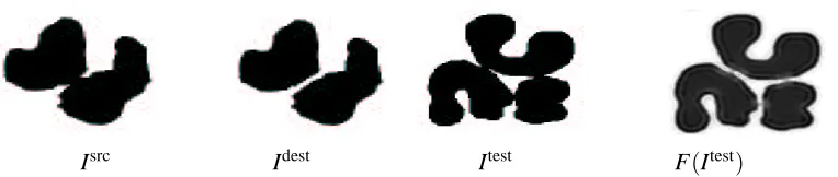
Figure 2: Results for the image transformation example. Images Isrc_{and I}dest_{where used for}

train-ing. Image Itest show the image for testing, the three connected should be separated. F(Isrc)shows the image after application of the trained image transformation.

We conduct two experiments. First we train the filter to separate connected clusters of pixels. The left two images in Figure 2 show the images Isrc, Idestused for training. As the equation system is highly overdetermined the regularization parameterγcan be chosen very small. If the training images are distorted by a small amount of independent Gaussian noise we can actually chooseγ=0. In general we can conclude that the higher the regularizationγis the less effective is our filter, but the more robust the filter is against additive noise. This is a well known behavior.

The right two images show a test image in its original appearance and after the application of the trained filter. One can see that the filter actually works properly. Of course, some artifacts are created. One can nicely see the equivariance of the filter. The behavior depends neither on the orientation of the touching areas nor the absolute position. In fact, the filter may be interpreted as a locally applied quadratic (because of the second-order polynomial kernel) Volterra filter. The test image Itest was chosen such that common methods would not work properly. For example, if one use a distance transform, the agglomerate would be divided in five instead three clusters, because the distance transform gives five local maxima.

As a second experiment we trained the filter to perform a deconvolution. For training we used a black disk on white background as target Idestand a blurred version as Isrc(blurred with a Gaussian of width 2 percent of the image size). In Figure 3 a) we show a blurred image which has to be sharpened (blurred with the same width as used for training). We compare our filter with an ordinary Wiener filter for deconvolution (see, for example, Jain, 1989). Assuming decorrelated Gaussian noise models, the Wiener filter only depends on the signal-to-noise ratio, which controls the intensity of the sharpening of the image. In our approach the regularization parameterγplays a similar role as the signal-to-noise ratio for the Wiener filter. We tuned the parameters such that the obtained sharpness for both approaches are visually comparable. In Figure 3 b) we give the result obtained by our method, in c) the result for the Wiener filter. Our method produces a more natural looking image and more importantly it produces no over- and undershoots at the sharp edges like the Wiener filter.

5.3 A Rotation Equivariant Object Detector

sharpened with Wiener filter

blurred original sharpend with equivariant filter

Figure 3: Results for the image restoration example. The Wiener filter produces overshoot- and undershoot-artifacts; this is a well known problem for inverse linear filters. Our non-linear filter creates a fine and accurate edge while having the same sharpness as the Wiener filter. (have a look at these results in an electronic form, a printer may destroy the fine differences)

which is learned from a shape template. It has also some similarities to the object recognition system using the so called SIFT features (Lowe, 2004).

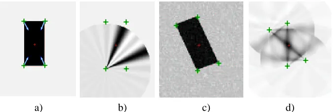
a) b) c) d)

Figure 4: Example for the rectangle. a) The rectangle with its four interest points and its center. b) The response of the trained voting function p(x) for the lower left interest point (as mentioned the distance to the center is not learned, only the direction). The function votes for the center of the shown rectangle and for the center of a putatively rotated rectangle by 90 degrees. c) an rotated version of the training object with additive Gaussian noise. d) the superimposed responses of all four interest points. The maxima is obviously in the center of the rectangle.

For simplicity we want to restrict ourselves to vote for points in the same specific direction with the same probability or weight, that is, the output of the equivariant-mapping is a probability distribution defined on the circle.

For the features we use the same projections on local basis-functions as in the previous exper-iment. To find the interest points we search for local maxima of the absolute value|[xz]2|, which

basically gives responses for corner-like structures. To eliminate responses at edges, which are rather unstable, we only take those local maxima whose values for the quotient |[xz]2|/|[xz]1|are

above a given threshold. Let x be a feature vector around some interest point andφthe angle to the center of the object. We are interested to learn the conditional distribution p(φ|x)from training sam-ples(φi,xi)belonging to the training object’s interest points. As we want to detect the objects in a

rotation invariant manner, the distribution has to fulfill rotation equivariance p(φ|g_ϕx) =p(φ+ϕ|x). In Section 4 we worked out that it is advantageous to work with irreducible kernels. As already men-tioned the irreducible kernels of the 2D-rotation group act on the Fourier representation of functions, so we denote p(φ|x)by the vector p(x), where its components are the Fourier coefficients of p(φ|x) in respect toφ. We denote the cutoff-frequency of the Fourier representation by N.

We do not rigorously model p as a probability distribution. Let e_φ be the unit-pulse in Fourier representation, then we minimize

∑

i

||eφi−p(xi)||2,

which is nothing else then the ordinary least-square regression scheme. But the solution basically behaves as we want it to. To get an idea, consider again the rectangle example with its four corners as interest points. If we neglect noise the local features xiof the corners are all the same xi=gϕix0

up to rotations g_ϕi of 0,90,180,270 degree. Then the equivariant least-square minimizer p(x0)is

proportional to the Fourier transformed histogram of the relative anglesφi+ϕi. The reader should

a) b)

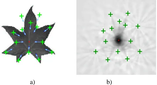
Figure 5: Training image a) The only training leaf. The interest points for training are marked and its corresponding direction to the center. b) The voting map for the training object. Black means high probability for the center, white low probability.

The scalar basis kernel is chosen to be the Gaussian kernel k(x1,x2) =e−λ||x1−x2||2_{. The diagonal} matrix kernel is approximated by using the FFT as depicted in Section 5.1. To get good approx-imations we have to perform frequency padding. In the experiments we used a FFT of size 6N (this is enough to compute a third-order polynomial kernel accurately). For accurate computation of the exponential kernel an infinite size FT would be needed, but the experiments have shown that an approximation is enough. The final learning procedure is very simple. We just have to solve N linear equations of the form

Knan=bn n=0, ...,N−1,

where the matrix entries of (Kn)i,j =Kn(xi,xj) are the approximations of Equation (7), and the

entries of the target are[bn]i=einφi.

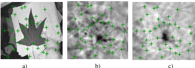
a) b) c)

Figure 6: A test image of a leaf with background and small clutter. a) The testimage with the found interest points. b) The voting map for test image with the simple matrix kernel. c) The voting map achieved with the enhanced kernel for better selectivity.

K0=K tr(K†K)to give it more selectivity to the features itself. In Figure 6 c) the voting map with this enhanced kernel is shown, the maximum seems to be much more robust.

6. Conclusion and Outlook

We presented a new type of matrix valued kernel for learning equivariant functions. Several prop-erties were shown and connections to representation theory were established. We showed with two illustrative examples that the theory is applicable.

The usage in nonlinear signal and image processing are apparent. Problems like image denois-ing, enhancement and image morphing can be tackled. Another simple task for the equivariant filter would be to gaps in road networks.

The proposed object detector shows in spite of its simplicity a nice behavior and generaliza-tion ability and should be worth to improve. Generalizageneraliza-tions of our proposed experiments to 3D-rotations are straightforward.

From a theoretical point an extension of our framework to non-compact groups would be satis-fying. Another important challenge is to find sparse learning algorithms with an unitary invariant loss functional. Unfortunately, the unitary extension of the ε-insensitive loss is not solvable via quadratic programming anymore. A last important issue is the local nature of transformations. In hand-written digit recognition invariance under rotations might turn a ”6” into a ”9”, while rota-tions by 5 degrees are ok. A generalization of our theory using norota-tions like approximate or partial equivariance are necessary.

Acknowledgments

References

L. Amodei. Reproducing kernels of vector-valued function spaces. In Surface Fitting and Multires-olution Methods, A. Le Maut C. Rabut and L. L. Schumaker (eds.), pages 17–26, 1996.

N. Aronszajn. Theory of reproducing kernels. Trans. AMS, 686:337404, 1950.

D.H. Ballard. Generalizing the hough transform to detect arbitrary shapes. Pattern Recognition, 13-2, 1981.

S. Boyd, L. O. Chua, and C. A. Desoer. Analytical foundations of Volterra series. IMA Journal of Mathematical Control and Information, 1:243–282, 1984.

J. Burbea and P. Masani. Banach and Hilbert spaces of vector-valued functions. Pitman Research Notes in Mathematics, 90, 1984.

H. Burkhardt and S. Siggelkow. Invariant features in pattern recognition - fundamentals and ap-plications. In In Nonlinear Model-Based Image/Video Processing and Analysis, pages 269–307. John Wiley and Sons, 2001.

N. Canterakis. Vollstaendige minimale systeme von polynominvarianten fuer die zyklischen grup-pen g(n) und fuer g(n) x g(n). In In Tagungsband des 9. Kolloquiums - DFG Schwerpunkt: Digitale Signalverarbeitung, pages 13–17, 1986.

T.J. Dodd and R.F. Harrison. Estimating Volterra filters in Hilbert space. In Proceedings of IFAC Conference on Intelligent Control Systems and Signal Processing, 2003.

A. Gaal. Linear Analysis and Represenatation Theory. Springer Verlag, New York, 1973.

B. Haasdonk, A. Vossen, and H. Burkhardt. Invariance in kernel methods by haar-integration ker-nels. In Proceedings of the 14th Scandinavian Conference on Image Analysis, pages 841–851, 2005.

A.K. Jain. Fundamentals of Digital Image Processing. Prentice-Hall, Inc., Englewood Cliffs, N.J., USA, 1989.

G.S. Kimeldorf and G. Wahba. Some results on Tchebycheffian spline functions. Journal of Math-ematical Analysis and Applications, 33:82–95, 1971.

R. Lenz. Group Theoretical Methods in Image Processing. Springer Verlag, Lecture Notes, 1990.

D.G. Lowe. Distinct image features from scale-invariant keypoints. International Journal of Com-puter Vision, 60:91–110, 2004.

C.A. Micchelli and M. Pontil. On learning vector-valued functions. Neural Computation, 17:177– 204, 2005.

W. Miller. Topics in harmonic analysis with applications to radar and sonar. IMA Volumes in Mathematics and its Applications, 1991.

L. Nachbin. The Haar Integral. D. van Nostrand Company, Inc., Princenton, New Jersey, Toronto, New York, London, 1965.

M. Pontil and C.A. Micchelli. Kernels for multi-task learning. In Proceeding of the NIPS, 2004.

V. I. Paulsen R. G. Douglas. Hilbert Modules over Function Algebras. Wiley New York, 1989.

M. Reisert and H. Burkhardt. Averaging similarity weighted group representations for pose estima-tion. In Proceedings of IVCNZ’05, 2005.

B. Schoelkopf and A. J. Smola. Learning with Kernels. The MIT Press, 2002.

I. Schur. Vorlesungen ueber Invariantentheorie. Springer Verlag, Berlin, Heidelberg, New York, 1968.